Nine narrated, beat-synced visual lessons, three per paper. Each opens in its own player: space to play, arrow keys for slides, comma and period to step through the beats of a figure, square brackets for speed, d for links into the notes and the PDF at the right page.
Every spoken sentence was fact-checked against the PDF pages by a skeptic agent before narration, and anything that is our inference and not the paper's is flagged out loud. The core lessons end with two recall questions; the player pauses itself before each answer.
Suggested path: the three core lessons first (about 27 minutes at 1×, 18 at 1.5×), then the deep dive that pulls at you, then the report pages under each paper, then the PDF.
What this is
Three PDFs from Omer Tamuz's Caltech page, surveyed on 2026-09-17. All three have Omer Tamuz (Caltech, economics and mathematics) as a co-author. They share an author and nothing else: one is pure math (amenability of a monoid), one is a lab experiment (social learning), one is economic theory with random-matrix tools (taxes and subsidies under noisy demand estimates).
These pages are a reader's survey: the goal was to get the core of each paper into one reader's head, fast, with the central points first and the logical next place to read after each. The notes were drafted in markdown and rendered into this page with compiled LaTeX. Survey agents wrote the notes and the report pages; nothing here was typed into the HTML by hand.
Status: pass 2. Seven survey agents have read every page of all three papers, including appendices and figures, and written the report pages that sit under each paper in the left rail. Their corrections to the pass 1 notes are merged. Every claim on these pages carries a PDF page link so it can be checked in one click. Page numbers are PDF page numbers (what the viewer's page box shows).
A regulator who sees the demand system through heavy noise can still raise total surplus with high probability, by subsidizing along the top eigenvectors of the Slutsky matrix. It works when those eigenvalues grow faster than the noise's operator norm.
People who see everyone's raw data and everyone's past guesses guess better than people who see the raw data alone, although the guesses add zero information. Imitation patches bad counting when the evidence is close.
The monoid generated by "delete the th entry" maps is amenable, although every finitely generated piece of it is non-amenable. Equivalently: random finite sets exist that barely change in law when you delete their th smallest element.
Pure math
27
Who Omer is, and where the papers stand
From public pages (agent C1, full map in tamuz-map): Omer Tamuz is a professor at Caltech, primary division HSS (economics) with PMA (mathematics) listed second. His homepage and the admissions office page say he chairs the undergraduate First-Year Admissions Committee.
All three PDFs are byte-identical to the public copies on his Caltech page, so none is a private draft. Status: the taxes paper is forthcoming in the Journal of Political Economy (arXiv 2411.03026); the imitation experiment is published in the Journal of Economic Theory 235 (2026); the face-maps paper is published in Math. Proc. Cambridge Philos. Soc. 181(1).
Suggested reading order
Taxes first. For a reader whose native tools are linear systems, eigenmodes and identification under noise, it is the closest to home, and about 80% of the value of the set sits here.
Learning experiment second. Fast to absorb, one clean result, one three-parameter model. It also bears on how to run multi-agent systems (should workers see each other's conclusions or only the raw sources).
Deletion last. Shortest paper, furthest from that background. The payoff is a clean idea (amenability that "hides at infinity") and a brush with Thompson's group , a famous open problem.
A loose common thread (the survey's reading, not the authors')
Each paper has a result that only appears in the large limit and fails at every finite stage.
Deletion: each finitely generated submonoid is non-amenable; the union is amenable.
Taxes: with finitely many products and bounded eigenvalues the regulator can do nothing robust; with and a top eigenvalue that outgrows the noise, robust intervention exists.
Learning: the weakest instance of the pattern. Group size helps only when raw signals are shared; with actions alone 8 people do about as well as 4, which the authors loosely connect to a bound that is uniform in group size.
This is a reading aid. It is not a claim the papers make.
How to use this page
Left rail or keys 123 jump to a paper. h is this hub, g the glossary, s how this was made. [ and ] step through sections. ? shows keys.
Dotted-underlined terms are glossary terms. Hover for the definition, click to open the entry.
Small p.N chips open the PDF at that page.
"Check yourself" boxes are closed by default. Answer in your head, then open.
The depth pills at the top of a paper page filter it: L0 one paragraph, L1 mechanism, L2 results ledger, L3 proofs and appendices.
paper
Robust Market Interventions
Andrea Galeotti, Benjamin Golub, Sanjeev Goyal, Eduard Talamàs, Omer Tamuz
field Economic theory, industrial organization, high-dimensional statisticsdated 2026-08-01 draft; per agent C1's web search (not in the PDF): forthcoming in the Journal of Political Economy, arXiv 2411.03026; subsumes "Taxes and Market Power: A Principal Components Approach" (arXiv 2112.08153)status pass 2 (whole paper read by two survey agents, reports attached; corrections from both merged here 2026-09-17; skeptic pass pending)open PDF (60 pp)
depth
LessonsL0 · core
Narrated, beat-synced visual lessons. Start with the core lesson, then go deeper where you want.
Reports behind the lessons: taxes-core (the argument, fully derived) and taxes-limits (Monte Carlo, Proposition 3, the diagnostic, hedonic models).
Core bitL0 · core
Claim. A regulator (or a marketplace operator like Amazon) sees the matrix of cross-price demand effects only through heavy noise. Entry by entry, the estimate is useless. The regulator can still pick per-unit subsidies and taxes that raise total surplus with probability near 1, provided the true matrix has a few very large eigenvalues and the noise has a small operator norm by comparison. p.2
Mechanism. Subsidize along a top eigenvector of the normalized Slutsky matrix. In that direction prices barely move, quantities move a lot, and each dollar spent returns about two dollars of producer surplus and about zero change in consumer surplus. Top eigenvectors survive noise (Davis–Kahan); the rest of the matrix does not need to be known. p.14p.19
Consequence. The policy-relevant object in a huge market is a low-dimensional subspace, and the condition for it to exist ("significant structure") requires large-scale complementarities across families of products. Models built mainly on substitutability, the usual focus in hedonic demand work, do not have it. p.5
The setup in control termsL1 · mechanism
A control-theory dictionary for this paper. The right column is the survey's translation, not the authors' language.
Paper
Control reading
firms, one product each, price competition (Bertrand)
-dimensional plant at an equilibrium operating point
Per-unit subsidy vector (negative entries are taxes)
small input around the operating point
Slutsky matrix , negative semidefinite
the plant Jacobian; symmetric, so it has an orthonormal eigenbasis
Price response (normalized units)
closed-loop DC gain
Signal ,
noisy system identification
"-robust": property holds with probability in every state
frequentist worst-case guarantee, no prior over plants (Wald)
a few high-gain modes whose gain outgrows the identification noise
Everything is first order. "" means the derivative of outcome in direction at . The paper never computes a finite intervention. p.7
Normalization: rescale units so every own-price effect is , that is . Then each firm's first-order condition reads , which is what makes the algebra short. p.10
Step 1. The budget identityL1 · mechanism
For any intervention, with consumer surplus, producer surplus, the regulator's spend: p.11
Read it as a frontier. If consumers are not to be hurt (), the most the regulator can buy is , reached when all the incidence goes to producers. Total surplus is , and the identity gives . So with consumers held harmless () the best rate is one dollar of net surplus per dollar spent. This is a full-information identity; nothing about robustness enters yet. Without the constraint on consumers the rate is unbounded: tax a low- mode and subsidize a high one at zero net spend. With full information, for generic , every surplus triple on the plane is reachable as long as has one nonzero off-diagonal entry (Proposition 1, part 2). p.11
Monopoly sanity check: one firm, linear demand. A subsidy drops the price by . Consumers get half the spend, the producer gets all of it (half on old volume, half on new volume). . p.11
Why information is the binding constraint: . The inverse is sensitive to every entry of . With a noisy the regulator cannot even sign . p.12
Step 2. Spectral price theoryL1 · mechanism
Write with eigenvalues . Think of eigenvector as a bundle of products. A subsidy proportional to moves only that bundle's price and quantity; the other bundles do not respond. Lemma 1: p.14
So per dollar spent in direction : consumers get , producers get , net total surplus is . p.19 Two forces oppose each other as grows. Strategic interaction among the firms makes the bundle's equilibrium price less sensitive to the subsidy. Demand for the bundle gets more sensitive to its price (the slope of bundle demand in bundle price is exactly , a fact about demand alone). The second force wins, so quantity pass-through rises with while price pass-through falls. p.14
try it · where one subsidy dollar goes, by eigenvalue of the mode you aim at
to consumers
to producers
net total surplus
Surplus effects add across modes, each weighted by how much status-quo quantity sits on that bundle (Lemma 2 on p.15, combined with Lemma 1 as equation (10) on p.20):
Put all of on modes with huge and : the frontier from Step 1. Two things must hold: is not orthogonal to those modes (otherwise the intervention spends nothing and does nothing), and the regulator can find them.
Step 3. Significant structure and recoveryL1 · mechanism
Definition 2. There is a threshold such that: p.16
quantity noise is no bigger than quantities, ;
demand noise is small next to the threshold in operator norm, ;
has eigenvalues above in absolute value, and keeps a fixed fraction of its norm inside their eigenspace.
Why this is plausible: for independent bounded-variance entry noise, grows like , while a matrix with complementarities of fixed size spread across categories has a top eigenvalue that grows like . The running example is a block model: products within a category are substitutes, across categories complements (tennis rackets and tennis shoes). In the homogeneous version its top eigenvector is exactly the all-ones vector and ; in the general block model Lemma 3 gives a positive, category-constant eigenvector. The noise bound needs independent, mean-zero, uniformly bounded errors. p.12p.17p.39
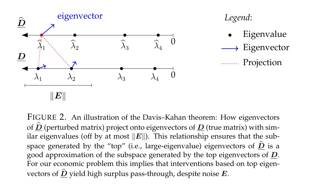
Recovery uses the subspace () form of Davis–Kahan, and it does not assume the large eigenvalues are separated from the rest of the spectrum or from each other. The proof manufactures its own gap with three thresholds: true eigenvalues above (the space ), estimated eigenvalues above (the computable space ), and true eigenvalues above (a buffer space ). Each comparison has a gap of , which dwarfs , so up to a vanishing tilt. No individual eigenvector is ever estimated. p.41p.42p.43 Full derivation: taxes-core.
The rule is a projection, so no sign is ever chosen: in normalized units. Estimated spend equals exactly. Quantity noise may be as large in norm as itself; it washes out because has at most dimensions (from and negative semidefiniteness), and independent noise spread over coordinates has almost no energy in so few. p.42p.44 The sign rule belongs only to the one-eigenvector sketch in the main text. p.20
Main theoremL2 · ledger
Theorem 1. Under significant structure and Assumptions 1 to 4, for any and target spend , for large enough a single rule achieves all of the following -robustly: (i) ; (ii) , and the same for every individual household; (iii) . p.18
The rule: normalize , project onto the span of eigenvectors of with eigenvalue above (the main text says ; the appendix proof needs the lower value), divide by the squared norm of the projection and multiply by . p.21p.42
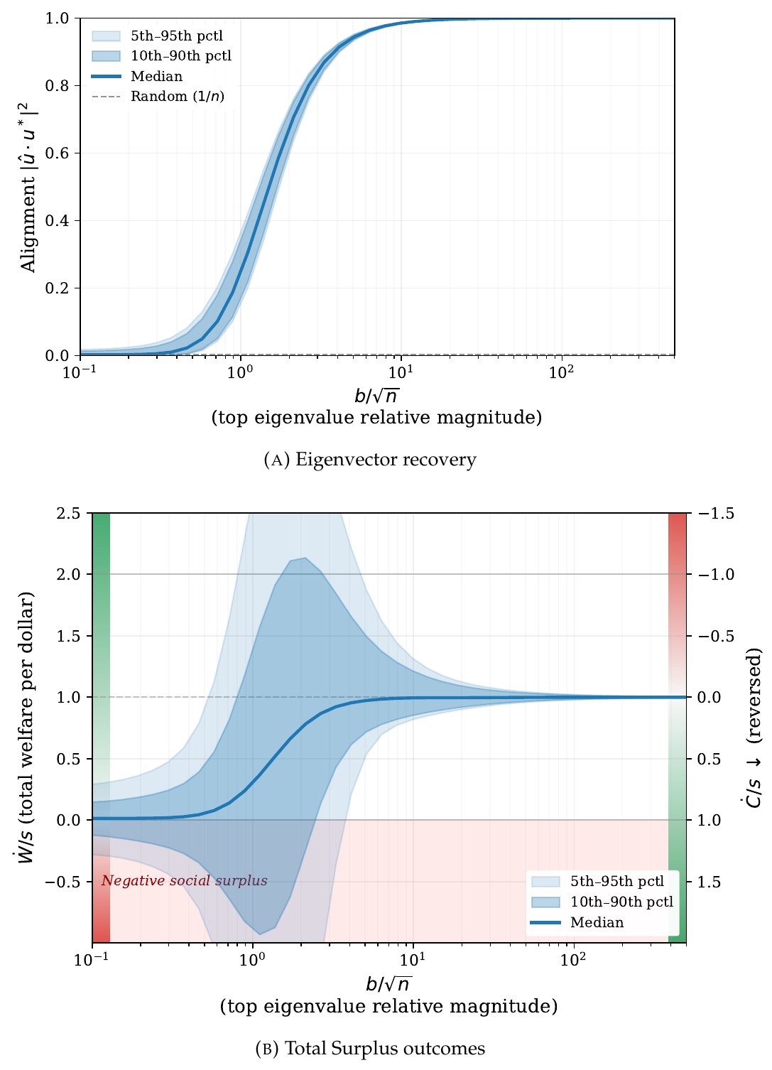
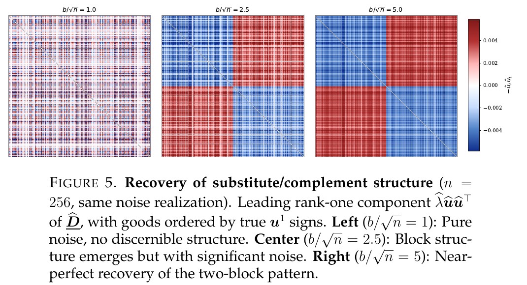
The figure to remember is the Monte Carlo in Section 7 (, two-block model with unknown block membership, Wigner noise). The horizontal axis is with ; the noise has operator norm about . Alignment and welfare-per-dollar switch on at . (Survey inference, confirmed by two independent re-simulations: that is half the noise norm and exactly the spiked-matrix (BBP) threshold, with squared overlap above it, and the Davis–Kahan bound is vacuous until about 4.) Reading Figure 3B: the 5th percentile of welfare is a loss from the left edge until about 3.7 and the 10th until about 2.4, including a stretch where the median is already above 0.5; the skeptic's re-run puts the share of losing runs at 42%, 18%, 7% at . The same band has a tail where consumers lose. Note the simulated example flips the sign pattern of Section 4: complements within blocks, substitutes across. p.22p.23p.24
Figure 3 of the paper: eigenvector recovery and total surplus per dollar against top eigenvalue over root n
Results ledgerL2 · ledger
Result
Statement, compressed
Page
Read?
Prop. 1
; full-information frontier is fully implementable
Constructed adversarial environments: (1) about states emit one signal; every rule's gain averaged over those states is , so in some state it earns at most that. The proposition bounds the guaranteed return (no rule robustly achieves ); it does not rule out improvement, and earns in every state of the construction; (2) the consumer-favoring direction has a statistically invisible sign. Neither shows impossibility under i.i.d. noise below threshold.
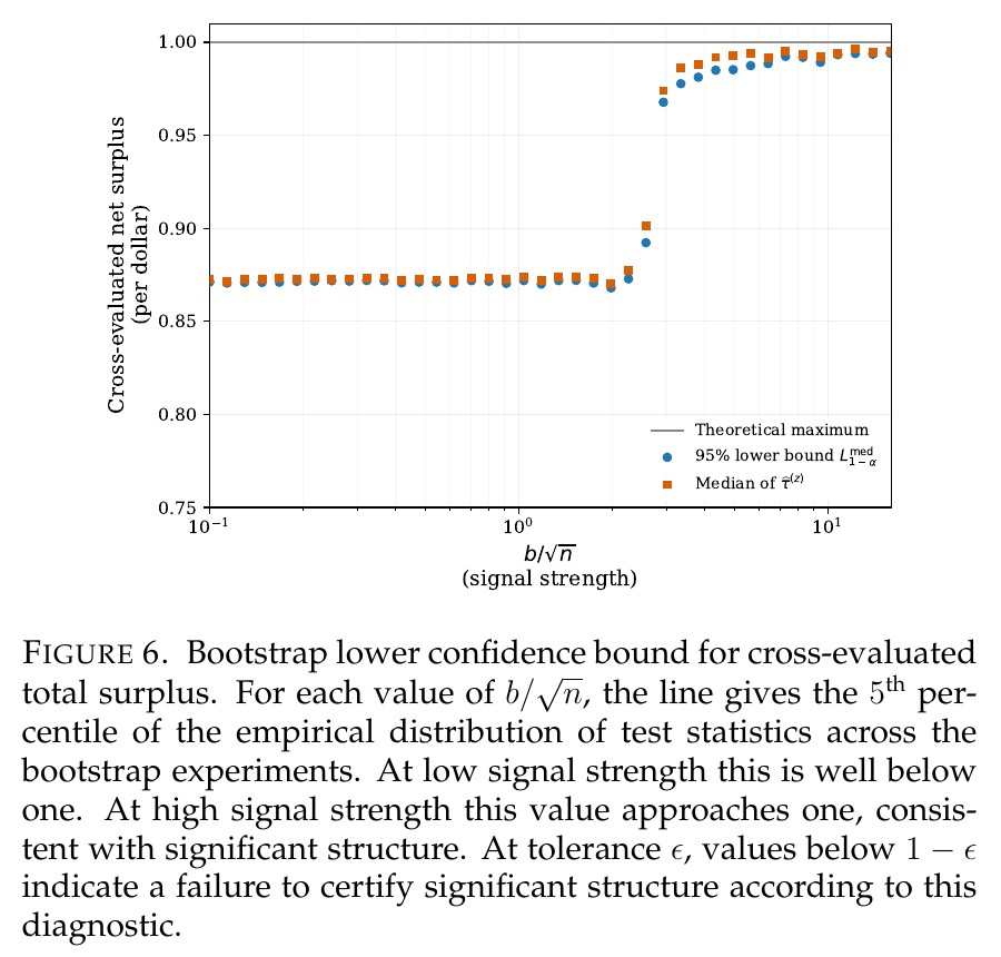
Diagnostic: cross-fit, score with Lemma 2 as if the second estimate were true, bootstrap a lower bound. T2 finds a noise floor near 0.87 at that the paper does not discuss.
This is "actuate only along well-identified high-gain modes." The full inverse is the fragile object; the top singular subspace is the robust one. The guarantee is worst case over plants and probabilistic only over the identification noise, which is the same split as in robust-control problems with stochastic sensor noise and an unknown-but-fixed plant.
bridge
Spiked random matrices
Confirmed by agent T2. In the paper's units the BBP threshold sits exactly at , and a re-run of Section 7 matches the overlap law to within 0.01 (the published Figure 3A is somewhat flatter, cause unknown). The paper uses the word "spike" and cites Davis–Kahan, Vershynin, Bandeira–van Handel and the Chen–Chi–Fan–Ma monograph, and cites no spiked-matrix paper. p.23p.36
Check yourselfL1 · mechanism
check yourselfA subsidy is aimed along an eigenvector with . Of each dollar spent, how much goes to consumers, producers, and net total surplus?
Consumers . Producers . Net total surplus . Check: , the budget identity.
check yourselfWhy can the regulator not just plug into and optimize?
The true operator is tame: is negative semidefinite, so every eigenvalue of is at least 1. The plug-in is the problem (survey inference, checked numerically by the skeptic). Noise of norm about makes indefinite, so has eigenvalues on both sides of zero and can be near singular (median smallest absolute eigenvalue 0.075 at ). The optimized would load on directions that look good only because of noise, and the sign of the true is not controlled. p.12p.14
check yourselfWhy does the definition of significant structure include a condition on the quantity vector ?
Two reasons. The spend in mode is , so if is orthogonal to the recoverable modes the intervention is a no-op. And the rule divides by , so the projection must stand clear of the projected quantity noise or the scale blows up (Lemma 5). p.43 In the one-eigenvector sketch the same condition is what lets the sign of be trusted. p.20
check yourselfWhy complements and not substitutes?
A short argument (from agent T2, not in the paper): if every off-diagonal entry is a substitute, write with entrywise. Negative semidefiniteness needs , and Perron–Frobenius gives . So every eigenvalue of lies in at any . Large eigenvalues need negative off-diagonal mass: complements. The paper's own argument runs on the utility Hessian: in hedonic models at Pellegrino's . p.60 Complements are needed somewhere, not everywhere: the Section 7 example has substitutes per good. p.22
Open questions for the surveyL3 · deep
A skeptic pass (taxes-verify) checked this note, the two reports and the core lesson against the PDF; its must-fix items are applied. Its one new observation: with observed exactly, weakly raises first-order welfare in every state with no knowledge of (from equation (9)), so what Theorem 1 buys is the rate, consumer neutrality and the spending target.
All eight are answered in taxes-core (questions 2 and 5) and taxes-limits (1, 3, 4, 6, 7). Question 8 (what the referees pushed on) was not pursued. One new criticism from T1: Appendix A.3 never invokes Assumption 4, and the normalization error is not automatically . p.41
Proposition 3, both parts: what exactly is impossible without significant structure, and why consumers cannot be robustly favored.
The no-gap subspace argument in Appendix A: what replaces per-eigenvector Davis–Kahan.
Section 8.2 diagnostic: statement, how it is computed, what it would take to run on real data.
Assumption 2 (own-price local linearity) and Section 8.4: how much breaks without it.
Which assumptions carry the "every household" clause of Theorem 1(ii).
Relation to Galeotti, Golub, Goyal (2020) "Targeting interventions in networks", which did the known-network version.
BBP question above.
What did the four referees likely push on? (Compare with the 2021 working paper if it can be found.)
Questions worth asking OmerL2 · ledger
Drafts after pass 1, to be sharpened or killed.
The guarantee is first order in . How large can the intervention get before the eigenbasis it was designed in has moved?
Is there an adversarial-noise version? The operator-norm condition seems to want independence across entries; a platform's estimates of would have structured errors.
Does significant structure show up in any real demand system you have looked at (the acknowledgments mention Pellegrino's data)?
paper
Learning Through Imitation: An Experiment
Marina Agranov, Gabriel Lopez-Moctezuma, Philipp Strack, Omer Tamuz
field Experimental economics, social learningdated 2026-05-17 draft; published in Journal of Economic Theory 235 (2026), article 106203; arXiv 2605.17662; NBER w29962; pre-registered as AEARCTR-0003315status pass 2 (whole paper and all appendices read by two survey agents, reports attached; corrections merged here 2026-09-17; skeptic pass pending)open PDF (84 pp)
depth
LessonsL0 · core
Narrated, beat-synced visual lessons. Start with the core lesson, then go deeper where you want.
Reports behind the lessons: learning-main (main text, every figure read) and learning-appendix (the 50-page appendix, audited).
Core bitL0 · core
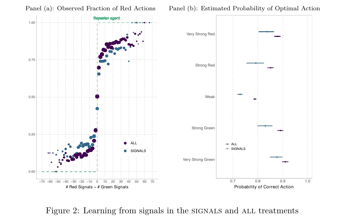
Claim. Give a group the full public record of evidence. Then also show them each other's past guesses. The guesses are a deterministic-or-noisy function of evidence everyone already has, so they carry zero extra information, and the standard behavioral worries (herding, correlation neglect, overload) predict they should hurt. They help: about 5 percentage points more correct guesses on average across rounds, and about 10 points more consensus. p.13 Read the first number with its uncertainty: Table A.1 gives 0.051 with a session-clustered standard error of 0.028 (significant at the 10% level, 11 sessions). The consensus effect, 0.095 with the same standard error, is the statistically firm one. p.34
Mechanism. People count evidence badly when the tally is close. In exactly those rounds they lean on what others did last round; when the tally is lopsided they ignore others. Other people's guesses are a noisy copy of the correct count, so mixing them in denoises your own. p.16p.17
Consequence. Imitation is a cheap error-correcting code on top of bad individual inference. Too much of it is still harmful (everyone copying everyone ignores the data), so the benefit lives at a moderate weight p.32, and the paper estimates that weight p.29.
The gameL1 · mechanism
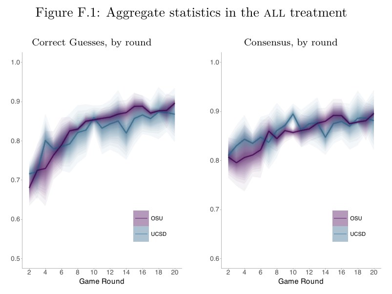
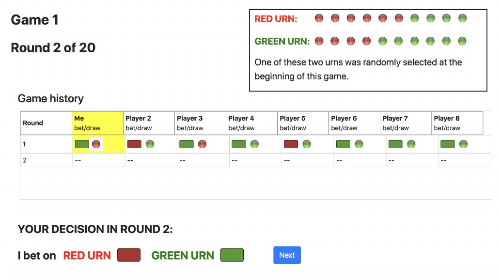
An urn is majority red (6 red, 4 green) or majority green, fair coin. Groups of 8. Twenty rounds. Each round every player guesses the urn's color, then gets one private draw with replacement, correct with probability 0.6. One random round of one random game pays $20 if correct and $5 if not, so there is nothing to hedge and myopic best-guessing is incentive compatible. Ten games per session, groups reshuffled each game. An on-screen table keeps the whole history, so memory is not a factor. 606 subjects, 31 sessions, UCSD lab and OSU online. p.6p.8
Four information treatments, all on top of your own signals: p.7
Treatment
See others' signals
See others' past actions
Group
Subjects
no info
no
no
1
80
actions
no
yes
8
136
signals
yes
no
8
82
all
yes
yes
8
152
actions4, all4
same as above
4
76, 80
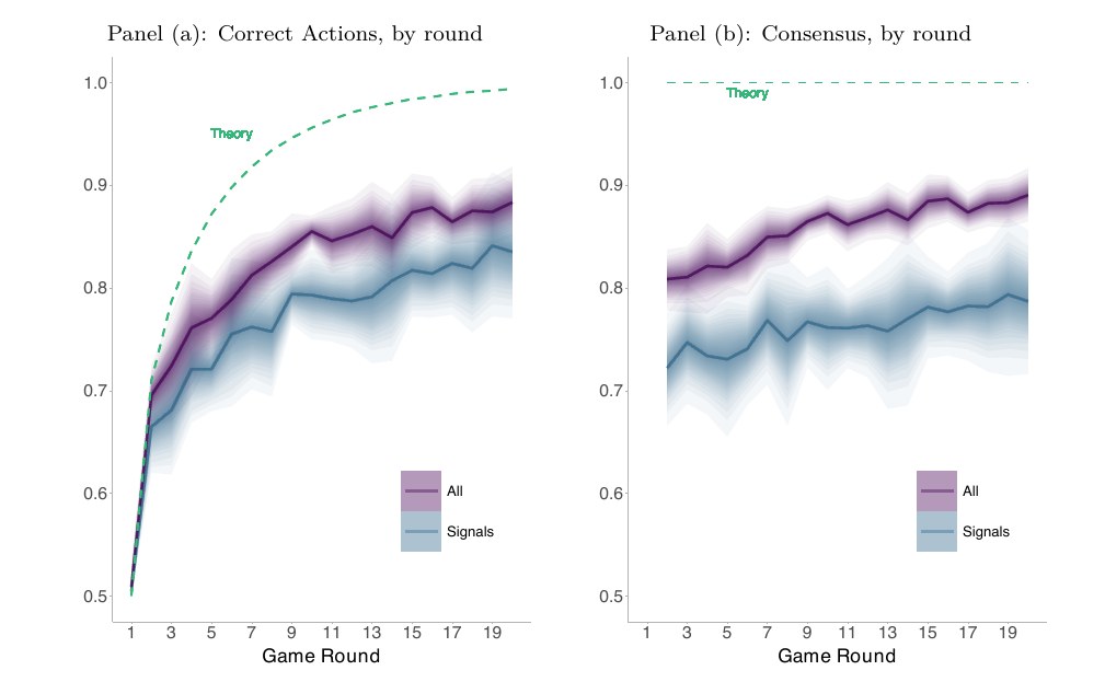
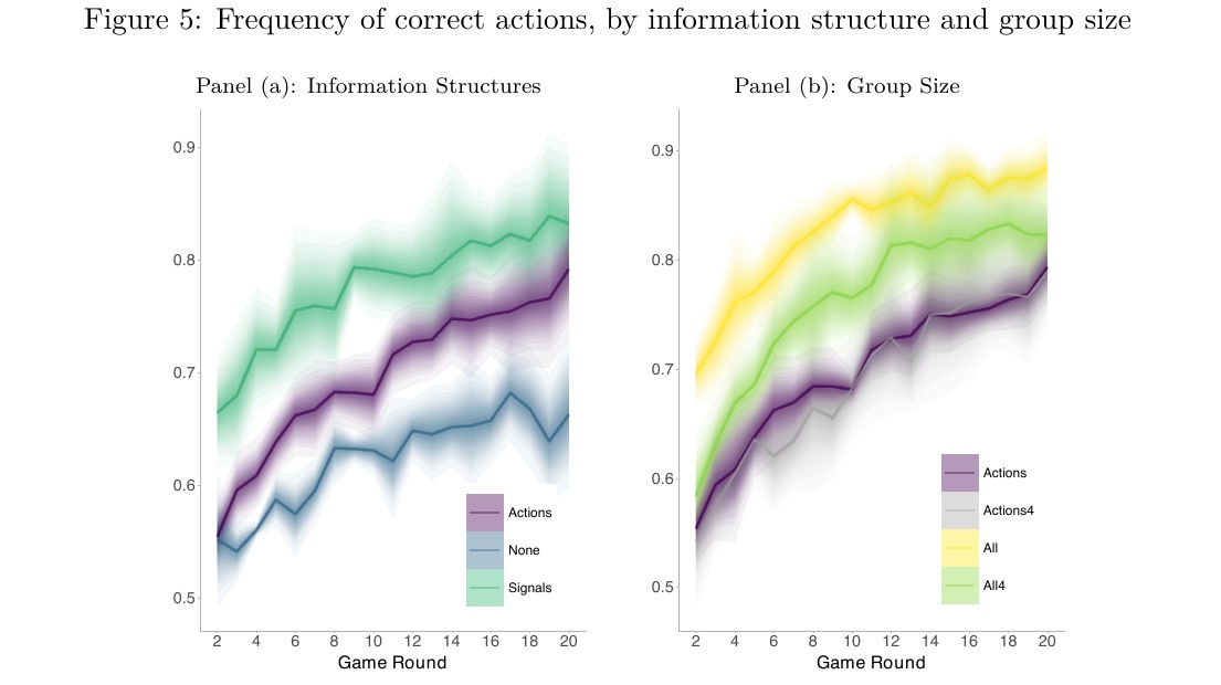
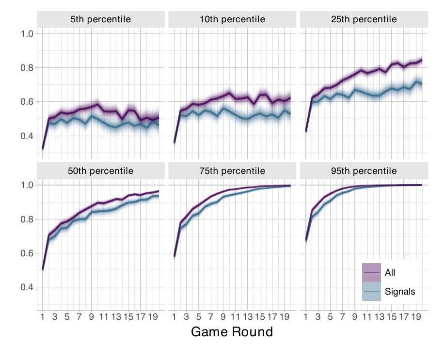
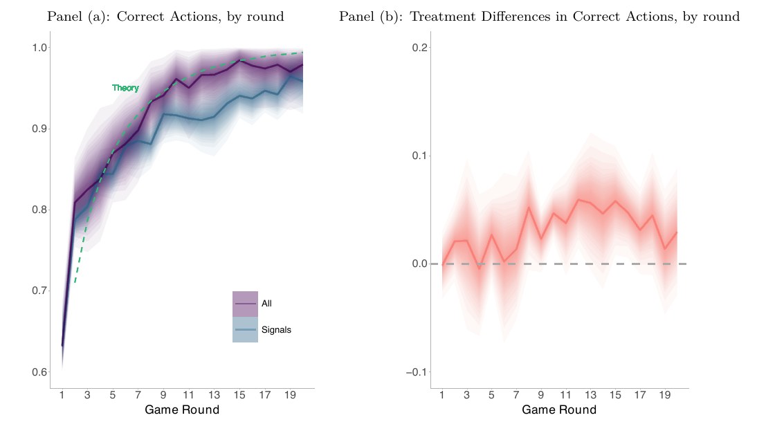
The headline comparison is signals against all. A Bayesian does identically in both: guess the color that is ahead in the pooled tally. The Bayesian benchmark hits 0.96 by round 10 and above 0.99 by round 18. p.10
What happenedL1 · mechanism
Figure 1 of the paper: share of correct guesses and consensus by round, all versus signals, with the Bayesian benchmark dashed
Both groups fall well short of the Bayesian curve, ending near 0.83 to 0.88 where theory says 0.99. The all group sits above the signals group from the early rounds on. p.12
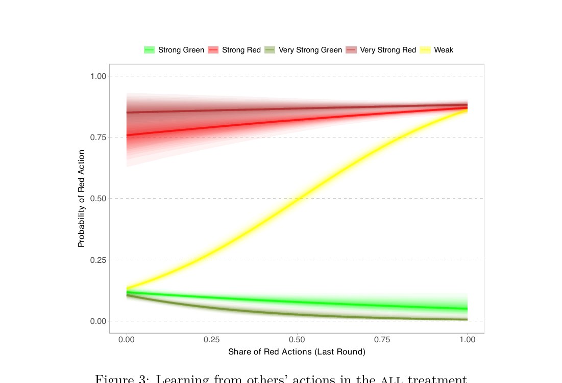
Figure 3 of the paper: probability of guessing red against the share of others who guessed red last round, by signal strength
This is the mechanism figure. Flat lines at top and bottom: when the pooled tally is lopsided, what others did has almost no effect on your guess. The steep yellow line: when the tally is close (difference within 14, the middle 50% of end-of-game histories; cutoffs on p.11p.12), your probability of guessing red runs from about 0.13 to about 0.86 as the share of others guessing red goes from 0 to 1. p.16 Caution from agent L1: inside the Weak bin the tally and the peers' share still move together, so this 0.73 swing overstates the causal effect. The structural model puts the effect of flipping one sampled peer at 0.31. The paper's own Figure 9 shows the same artifact. p.30
The paper's four numbered observations, compressed:
Seeing signals and actions beats seeing signals alone, in accuracy and in consensus. p.14
In both treatments people use the signals worse than a Bayesian would, mostly when the tally is close. In all they patch those errors with others' actions. p.17
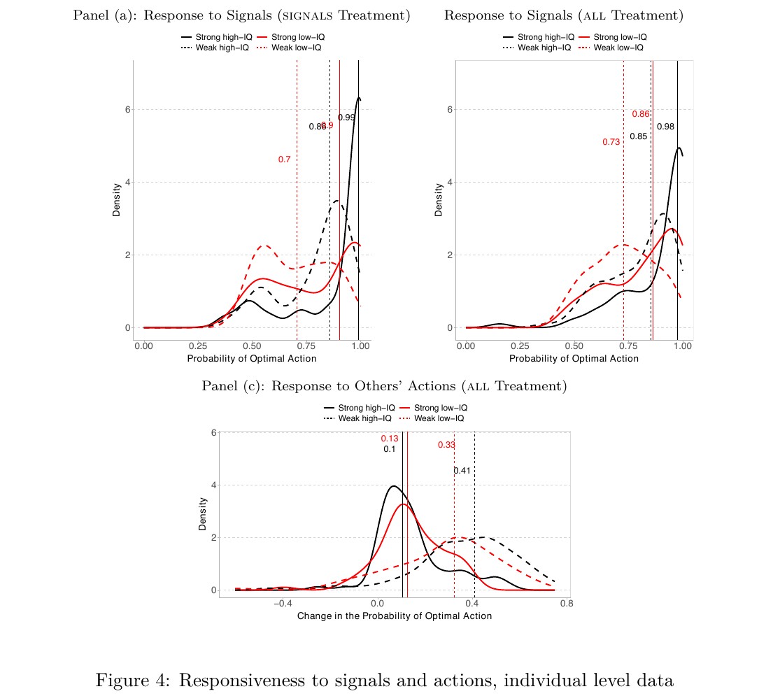
High-IQ subjects (six ICAR items) process the raw signals well with or without social information. Low-IQ subjects do not, and do badly without it. Both groups condition on others' actions, almost only when signals are weak, and both gain. p.20 The low-IQ gain is no larger than the high-IQ gain (interaction +0.010, SE 0.031, Table J.2). p.64
With signals and actions visible, groups of 8 learn faster than groups of 4 (all minus all4 = 0.065, SE 0.023). With actions only the difference is 0.008 (SE 0.022). p.35 The authors link this to Harel, Mossel, Strack, Tamuz (2021, "Rational Groupthink"), and call the link "quite a loose interpretation" themselves. p.22 The interval for the actions effect also contains the 0.04 to 0.05 gap that myopic Bayesians would show (Table 2), so the data cannot separate "no effect" from "the Bayesian effect".
Private-information side result: actions beats no info by a wide margin (the footnote gives 5.3 points early, 9.6 points late), although extracting private signals from repeated actions is a hard inference problem in theory. p.22
The three-parameter modelL1 · mechanism
Each round, player looks at two numbers. is the pooled signal tally (red , green ) divided by the number of signals raised to a power . is the last-round action of one randomly chosen other player. The player guesses red with logistic probability: p.22
That is the likelihood used for estimation in Section 6.2, where the sampled peer is latent and integrated out against the share of others who guessed red. p.26
check this
A units inconsistency between Section 6.1 and Section 6.2 (found in pass 1, ruled on by agent L1)
Section 6.1 describes the choice rule as "probability proportional to " and simulates at . Section 6.2 estimates with , and Table 3's probability effects pin that scale exactly: . p.29 L1 re-simulated 20,000 games per cell against eleven read-offs from Figures 6 and 7. The curves with no imitation match only with doubled. The imitation curves fit an effective of 0.8 to 1 and reject 2. So in Table 3 units the illustration is about , close to the estimates. the survey's first reading (both doubled, "subjects imitate far less than the illustration") was half right and its conclusion is withdrawn. Details: learning-main.
is the Bayesian sufficient statistic (raw difference). is the sample proportion, the usual choice in the behavioral literature. Estimates land between 0.52 and 0.63, which the paper calls closer to a square-root scaling than to the sample proportion (0.5 itself lies outside the credible intervals for signals and all): two reds alone feel stronger than 102 reds against 100 greens, but less drastically than proportion-thinking implies. p.23p.28 L1 adds that may be absorbing inattention: the model has no lapse rate, and about a quarter of subjects in two treatments act as if random (Appendix N).
Parameter
no info
signals
actions
all
(weight on tally)
1.05
1.02
1.27
1.27
(weight on a peer's last action)
0.97
0.65
(tally normalization)
0.52
0.57
0.52
0.63
Posterior medians from Table 3. In all, flipping the sampled peer from green to red moves by 0.31, about the same as a one standard deviation move in (0.29). p.29
Why helps here: the mistake probability depends on the sign and size of . is correlated with the sign of because peers mostly follow the tally. Adding it usually pushes the sum the right way, and it matters most when , where your own response is close to a coin flip. p.24
Survey replication, 3,000 simulated games at the Table 3 medians: all ends at 0.86 and signals at 0.83 in round 20, close to the data in Figure 1. Holding and at the all estimates and sweeping , round-20 accuracy climbs from 0.82 at to about 0.90 on a flat top from 1.75 to 2.6, then collapses (0.68 at ). Under the paid objective (mean accuracy over rounds) the optimum is about 1.5 and the gain over the subjects' 0.65 is about 2 points (skeptic re-run, 80,000 games per point). That is a simulation by the survey on the paper's model, and the paper does not claim it.
try it · the three-parameter model, simulated in your browser (2,000 games per curve)
sees signals and actions (your ) sees signals only () Bayesian benchmark
Bridges to adjacent fieldsL1 · mechanism
bridge
Noisy decoders and a redundant channel
Each subject is a noisy decoder of a sufficient statistic. A peer's action is the output of another noisy decoder of the same statistic. No new information about the urn enters, yet averaging two noisy decodes of one codeword lowers decode error. The Bayesian argument "actions are redundant" assumes a noiseless decoder. This is the whole paper in one sentence, and it is the survey's phrasing, not the authors'.
bridge
Multi-agent systems (speculation)
The same design question arises when fanning out AI subagents: do workers see only the raw sources, or also each other's conclusions? For humans this paper says conclusions help, most when evidence is close; the gain is no larger for low-IQ subjects p.64 and is largest for the lower quantiles of realized performance p.72; and that the help saturates with group size unless raw data is also shared. A common operating rule for LLM workers (never treat another agent's summary as a source) points the other way, because a wrong summary is copied with confidence. The paper's own caveat applies: too much weight on others is harmful, and it never tests a confidently wrong peer. The discussion section names that as future work ("ideological agents whose actions are independent of the data"). p.32
bridge
Self-consistency in LLM sampling (speculation)
Majority vote is not a corner of this model (corrected by the skeptic). At and large each player copies one randomly sampled peer, which is a voter-model step with no pull toward the majority. The analogue of self-consistency would be a variant that responds to the share of peers through a threshold, which the paper does not study.
Check yourselfL1 · mechanism
check yourselfWhy would a Bayesian do exactly as well in signals as in all?
In both she sees every signal ever drawn. Others' actions are functions of those same signals (plus noise that is independent of the urn), so conditioning on them cannot change her posterior.
check yourselfIn Figure 3, why are the top and bottom lines flat while the middle one is steep?
With a lopsided tally, dominates and the guess follows the data whatever the peers did. With a close tally and the term decides.
check yourselfGroup size helps in all and does nothing in actions. One sentence why.
In all, a bigger group means more raw draws per round in the shared tally. In actions, more peers mostly means more copies of correlated guesses, and the information that can be squeezed out of actions saturates (Harel et al. 2021).
check yourselfWhat does mean in plain words?
People weigh a lead of signals out of roughly like . That happens to be the scale of a z-score for the tally, so subjects behave as if judging "how many standard deviations ahead is red". (The z-score remark is the survey's, not the paper's.)
Audited in learning-appendix: effect sizes with SEs (A), stated strategies (B), beliefs (C), instructions and screenshots (D, E), lab versus online (F), learning across games (G), cutoff robustness (H), RMSE value of actions (K), heterogeneity (L), covariate balance (M), random-acting subjects (N)
A skeptic pass (learning-verify) checked this note, both reports and the core lesson against the PDF, re-ran the units ruling (agrees: doubles, does not) and the sweep. Two facts it added: the paper's subject-level measure finds high-IQ subjects rely on others more () p.20, and Appendix L finds the treatment effect largest in the lower quantiles of realized performance p.72.
Answered in learning-main (1, 5, 7) and learning-appendix (2, 3, 4, 6). The short version of the audit: the lab-versus-online confound is never directly tested (Appendix F compares only all at UCSD with all at OSU and prints no numbers; L2's digitized within-online gap is about 5.4 points, with no usable standard error; by subjects all is 64 UCSD and 88 OSU); Appendix N covers only no info and signals and never re-runs the headline without the random-acting quarter; the screen shows no running tally, so part of the counting noise comes from the interface (agent inference). p.8p.51p.56
Exact model normalization and estimation (Section 6.2): hierarchical? per-subject? How was "one random peer" handled in the likelihood?
Is the +5 point effect robust to the lab-versus-online split? Signals ran only online at OSU; all ran half in the UCSD lab, half online. That is a confound worth reading Appendix F for. p.8
Appendix K: how much of the gap to the Bayesian benchmark does imitation close, in RMSE terms?
Appendix N: how many subjects are effectively random, and do results survive dropping them?
Is there an optimal ? the survey's sweep says yes, near 2 for . The authors mention a formal analysis and conjectures as future work; find where and what, and whether they note that subjects under-imitate.
What do subjects say they did (Appendix B, open-ended strategies)?
Observation 3 details: size of the low-IQ gain.
Questions worth asking OmerL2 · ledger
Drafts after pass 1.
With a peer who is confidently wrong on purpose, where does the benefit of imitation break? (They flag this as future work.)
Does the normalization suggest subjects are doing significance testing in their heads?
For a fixed decoder noise , what maximizes group accuracy, and do subjects sit near it?
paper
A Fixed-Point Theorem for Face Maps, or Deletion-Tolerant Random Finite Sets
Tom Hutchcroft, Nicolas Monod, Omer Tamuz
field Pure math (amenability, semigroups, ergodic theory)dated compiled 2025-06-25; arXiv 2505.21484v2; published in Math. Proc. Cambridge Philos. Soc. (per agent D2's web search; volume and pagination unresolved)status pass 2 (whole paper read by two survey agents, reports attached; corrections merged here 2026-09-17; skeptic pass pending)open PDF (27 pp)
depth
LessonsL0 · core
Narrated, beat-synced visual lessons. Start with the core lesson, then go deeper where you want.
Reports behind the lessons: deletion-proofs (line-by-line proof read) and deletion-context (Appendix B, amenability, Thompson's , Moore, Ryll-Nardzewski).
Core bitL0 · core
Claim. Take a finite set of integers and delete its th smallest element; call that map . For any and any there is a finitely supported random finite set whose law moves by less than in total variation under every one of (Theorem A). The companion result: any infinite family of continuous affine maps of a compact convex set that satisfies the face relations for has a common fixed point (Theorem B). The paper calls the two "two visages of the same phenomenon" and derives both from one idempotent mean; it does not claim they are equivalent statements. p.3p.1p.2
Mechanism. Build a "random walk" whose step distribution is an idempotent mean on , a finitely additive probability measure sitting at infinity with . Deleting any entry of its -point trajectory gives exactly its -point trajectory, because merging two adjacent steps is a convolution and the convolution changes nothing. Then approximate that impossible object by honest finitely supported distributions using Day's Hahn–Banach argument. p.5p.6
Consequence. The monoid presented by the face relations is amenable. Each submonoid generated by with is non-amenable. For groups that cannot happen, since every subgroup of an amenable group is amenable. The authors' phrase: the amenability of "hides at infinity." is a quotient of the positive monoid of Thompson's group , whose amenability is a famous open problem. p.2p.3
Why the two theorems are one theoremL1 · mechanism
Day's theorem: for a monoid the following are equivalent. (1) Every action of by continuous affine maps on a nonempty compact convex set has a fixed point. (2) has a left-invariant mean. (3) For every finite and there is a finitely supported probability on with for all . p.12
Theorem B is (1). Theorem A is the same kind of statement as (3), for the deletion maps acting on finite sets. Precision from agent D1: the paper proves Theorem A directly on finite sets in Section 2 and never passes through ; Sections 3 and 4 exist to move the same mean onto and get Theorem B. The identification of with finite sets:
Every element of has a unique flat normal form with (rewrite until stuck; termination and local confluence, then Newman's lemma). So as a set. p.10
Under that identification, left multiplication by is : fill the th hole of the set (adjoin the th smallest integer not in it). p.11
Taking complements inside swaps "fill the th hole" with "delete the th element" on a suitable class of sets ("pin-headed": nonempty, and ). p.7p.8
So the level-lowering means become level-lowering means for hole-filling, and a Cesàro limit over all levels is a left-invariant mean on , which is amenability. p.9
try it · deleting entries and filling holes are the same action seen through a complement
pin-headed set (gold). Buttons apply : delete the th smallest element.
its mirror (blue). Buttons apply : fill the th hole.
The proof of Theorem A in five movesL1 · mechanism
Pick . Take any invariant mean on (an accumulation point of uniform distributions on , equivalently a Banach limit flavored Cesàro limit). It satisfies : convolving it with itself gives it back. It gives mass zero to every finite set, so think of it as "a random very large number." p.4p.5
Walk. Define on increasing -tuples by iterating: with . Loosely, is the law of the first positions of a walk with i.i.d. steps. Only loosely: Fubini fails for means, and the definition is the (non-commutative) Arens product. p.4
Theorem 2.3: for every . Deleting the last position obviously gives the -step walk. Deleting position in the middle merges steps and into one step of law , so again a -step walk. The written proof is this idea done carefully with the order of the nested means respected, plus an induction for . p.5p.6
Average over . is within of each . An accumulation point is exactly invariant under . p.6
Come back to earth. Finitely supported probabilities are weak-* dense in means (Goldstine). Weak convergence of upgrades to norm convergence after passing to convex combinations (Mazur's trick, which is Hahn–Banach). Norm in is twice total variation. p.6p.7
What is lost: constructiveness. The proof uses choice-type arguments several times (D1 counts at least four) and gives no rate. With a genuine countably additive step law the walk cannot work: stays at total variation distance more than from (Proposition A.1). The introduction says an explicit construction could be verified only for , but that verification is written nowhere in the paper; Appendix A offers a conjectural tower-of-exponentials model and says closeness holds for marginals, pairs and triples. p.3p.19p.20p.21 D1 also notes the mean "walk" is scale-ordered (the first step exceeds the second with mean-probability 1), which no i.i.d. walk can imitate; see deletion-proofs.
The Polish monoids of order-preserving maps of are amenable as topological monoids (a dense amenable submonoid suffices) and non-amenable as abstract monoids (the "waltz" map on diffuse means forces )
Exchangeability (survey observation, confirmed by agent D2)
Proposition 6.1 looks like the Ryll-Nardzewski theorem in different clothes. A law on sequences that is invariant under deleting any coordinate is what probabilists call contractable or spreadable, and Ryll-Nardzewski (1957) showed spreadable is the same as exchangeable, so by de Finetti it is a mixture of i.i.d., and the ergodic ones are i.i.d. The paper calls its result "a De Finetti type theorem" and the text dump contains neither "Ryll", "spreadable", "contractable" nor "Kallenberg". D2's ruling: deletion invariance is exactly contractability (finite-dimensional marginals suffice, no approximation needed), none of the paper's 17 references is on exchangeability, and the proof adds one thing: it needs no standard-Borel hypothesis on the state space. See deletion-context.
bridge
Stationarity under thinning
For an engineer the picture is a point process on whose law does not change when you drop its th point. A renewal process with i.i.d. gaps is invariant under dropping a point only if the sum of two gaps has the law of one gap, which no real distribution satisfies. The proof gets around this with a gap law that lives at infinity, then pulls back an approximation. The lower bound says any honest renewal process is a bad approximant, so the good finite approximants must look quite different from a renewal process. What they look like is open.
bridge
Simplicial objects
for are the face-map identities of a simplicial set, with all dimensions glued into one monoid. Theorem A then says: an infinite-dimensional simplicial complex carries random simplices that are almost invariant under passing to a face. p.2
Check yourselfL1 · mechanism
check yourself. Compute and . Which face relation do you see?
Maps compose right to left. : first , then gives . : first , then gives . They differ, so the maps do not commute. The face relation (for ) repairs the order: with it says , and indeed , then gives . Reason: once the th element is gone, what used to be the th element sits in position .
check yourselfWhy can a true probability distribution on never be convolution-idempotent?
If are i.i.d. positive integers then always, so cannot have the law of . (The paper notes that on the only finitely supported idempotent is the point mass at 0.) A mean can be idempotent because it gives zero mass to every finite set, so "adding a very large number to a very large number" is again just "a very large number."
check yourselfWhy is non-amenable?
On any compact convex with two points , let be the constant map to and the constant map to . Every truncated relation has , so the outer map on each side is one of and both sides are the constant map to . The only fixed point of is and the only fixed point of is , so there is no common one. Lemma 4.4 is needed to know these truncated relations are all the relations in .
check yourselfWhere does the argument use that there are infinitely many generators?
In , the relation always has room for . Invariance under is bought by pushing the defect out to higher and higher indices (the Cesàro average over in move 4), and there is always a higher index to push to.
Open questions for the surveyL3 · deep
Answered in deletion-proofs (1, 3 in part, 6, 7) and deletion-context (2, 3, 4, 5, 7). Two corrections to what is written below. Moore's two cited papers are a conjecture and its refutation: [Moo15] showed an idempotent mean on the free nonassociative magma would make amenable, and [Moo19] proved no such mean exists; the "echo" is that this paper runs the same idempotent-mean strategy on the associative , where idempotents do exist. And the direction of inference: is a quotient of , so amenability of would imply Theorem B and not the reverse. D1 also found three small slips in the paper (an off-by-one in the factor map of Prop. 6.3, a subscript on p.17, a plus sign for a product on p.20).
Appendix A: the conjectural explicit model, and the verification.
Theorem B.1 proof: why topological amenability but not abstract amenability.
Proposition 5.3 and the Klawe reference: the asymmetric Følner phenomenon in one paragraph.
Moore's work on ([Moo15], [Moo19]) and what "echoes" means on p.3.
The Ryll-Nardzewski question above.
Is there any quantitative version of Theorem A? How large must the support be as a function of ? The paper says none is known. p.7
What would amenability of need beyond Proposition 5.5? Why does the embedding into an amenable monoid not finish the job? (Submonoids of amenable monoids need not be amenable. This paper's own is an example. Confirm that is the whole obstruction.)
Questions worth asking OmerL2 · ledger
Drafts after pass 1.
What do the almost-invariant random sets look like? The bound kills renewal processes; is there a guess for ?
Is Proposition 6.1 Ryll-Nardzewski, and if so was the proof the reason to include it?
Did this come out of a probability question (the title's second half) or out of (the first half)?
report
Omer Tamuz, a map of the research program
status web survey on 2026-09-17 of his Caltech homepage, Caltech HSS and admissions pages, arXiv listings (81 entries), Crossref, Cambridge Core and the Math Genealogy Project; public PDFs hashed against the surveyed copies; no paper proofs read here
How to read this page
Every factual claim links to the public page it came from; this report has no PDF of its own, so links replace page chips. "(agent inference)" marks my own reading. Result statements are compressed from public abstracts. I read no proofs for this report.
Provenance finding: the three PDFs are the public copies
The three surveyed files are byte-identical to the PDFs on his homepage. I downloaded taxes.pdf, learning_experiment.pdf and deletion.pdf and compared MD5 hashes with the surveyed copies. All three match (taxes 632481f0..., learning 505f07d1..., deletion 2c0ec1af...). The hub's worry that these might be private drafts is settled: they are public postings. The PDFs carry no confidentiality.
1. Who he is
Appointment. Professor of Economics and Mathematics at Caltech, in the Division of the Humanities and Social Sciences. He was Assistant Professor 2015 to 2019 and Professor from 2019 (HSS page). The same page lists him as a member of the Division of Physics, Mathematics and Astronomy, the Linde Institute, the Center for Social Information Sciences (CSIS) and the Center for Theoretical and Experimental Social Sciences. The CMS department page also carries a profile with the same title. His office is Baxter Hall 213 (homepage).
Admissions role. Found. His homepage says he is "the chair of Caltech's undergrad admissions committee" and links to the admissions office's faculty page (homepage). That page names him as "Chair, First-Year Admissions Committee" and says more than 20 faculty do full reviews of applications after staff review (Caltech admissions). The HSS page repeats the role. This matches the "Omer" in the hub's open identity question on title and on the PMA membership. Note the public title is First-Year admissions. I found no public page that ties him to transfer admissions specifically.
Training. B.Sc. in computer science and physics, Tel Aviv University (2006), where he worked on extrasolar planet searches with Tsevi Mazeh. M.Sc. (2010) and Ph.D. in mathematics (2013) at the Weizmann Institute, advised by Elchanan Mossel (homepage, HSS page). Thesis title: "Learning, Agreement and Computation on Social Networks" (Math Genealogy). Schramm postdoctoral fellow at MIT mathematics and Microsoft Research, 2013 to 2015, after an internship with Adam Kalai at Microsoft Research (homepage). His list also has astronomy papers from 2005 to 2010 and two ICML papers with Kalai.
Awards and support. Sloan research fellowship in mathematics, NSF CAREER award (DMS-1944153), a MURI grant, a BSF award, a Simons Foundation award. Paper prizes: EC'20 best paper for "Feasible joint posterior beliefs" and MATCH-UP 2024 best paper for "The power of two in token systems" (homepage).
Students. Math Genealogy lists three PhD students: Pooya Vahidi Ferdowsi (2020), Joshua Frisch (2021), Michael Wolman (2025) (Math Genealogy). The first two co-wrote the Annals paper below.
Editorial roles. Not found. His homepage lists none. He does not appear on the current Econometrica editorial board or the current Theoretical Economics board. I found no public CV. A search engine summary asserted associate editorships with no source page behind it; I discard it.
2. The research program in seven threads
The homepage's own description: "probability, dynamics and group theory, and in their applications to topics in microeconomic theory, including information, risk and uncertainty, and social choice" (homepage). All venue and year data below come from that page's publication list.
Thread A. Social learning and information aggregation
Recurring idea: agents who watch each other's actions (coarse functions of beliefs) recover only part of what the group knows, and the question is how much, how fast, and on which network.
Asymptotic learning on Bayesian social networks (Mossel, Sly, Tamuz; Probability Theory and Related Fields 2014). Bayesian agents on a graph repeatedly see neighbors' best guesses of a binary state; the paper gives sufficient conditions on graph families under which, with probability tending to 1, everyone ends up correct, and counterexamples when the conditions fail (arXiv 1207.5893).
Strategic learning and the topology of social networks (Mossel, Sly, Tamuz; Econometrica 2015). With strategic agents, a geometric "egalitarianism" condition on the network guarantees learning in every equilibrium, and non-egalitarian networks have equilibria where learning fails (arXiv 1209.5527).
Rational groupthink (Harel, Mossel, Strack, Tamuz; QJE 2021). See section 3(b). Extended to networks and forward-looking agents in Learning in repeated interactions on networks (Huang, Strack, Tamuz; Econometrica 2024): in any equilibrium, on any network, for any patience, the speed of learning is bounded by a constant that depends only on the private signal distribution (arXiv 2112.14265).
Two surveys frame the thread: Opinion exchange dynamics with Mossel (Probability Surveys 2017, written for mathematicians, arXiv 1401.4770) and Information cascades and social learning with Bikhchandani, Hirshleifer and Welch (Journal of Economic Literature 2024, arXiv 2105.11044).
Thread B. Random walks on groups, boundaries, and strong forms of amenability
Recurring idea: classify groups by whether some averaging object at infinity is trivial. A bounded -harmonic function is a function on the group with ; the Poisson boundary is the space that parametrizes all of them, and it is trivial exactly when they are all constant.
Choquet-Deny groups and the infinite conjugacy class property (Frisch, Hartman, Tamuz, Vahidi Ferdowsi; Annals of Mathematics 2019). A countable group has only constant bounded harmonic functions for every non-degenerate step distribution if and only if no quotient has the infinite conjugacy class (ICC) property, meaning every non-identity element has infinitely many conjugates; for finitely generated groups this is the same as virtually nilpotent (arXiv 1802.00751). The arXiv listing says 14 pages.
Strong amenability and the infinite conjugacy class property (Frisch, Tamuz, Vahidi Ferdowsi; Inventiones 2019). A group is strongly amenable if every proximal action on a compact space has a fixed point; the same ICC criterion characterizes it (arXiv 1801.04024).
Thompson's group F is not strongly amenable (Hartman, Juschenko, Tamuz, Vahidi Ferdowsi; Ergodic Theory and Dynamical Systems 2019). They build a proximal action of on a compact metric space with no fixed point (arXiv 1607.04915).
Thread C. Entropy, stationary measures and ergodic theory
Recurring idea: entropy as a numerical invariant of a random walk or a group action, and the question of which values and which measures can occur.
Generic stationary measures and actions (Bowen, Hartman, Tamuz; Transactions of the AMS 2017). For a finite-entropy walk, a generic stationary measure on a shift space is an essentially free extension of the Poisson boundary (arXiv 1405.2260).
On the spectrum of asymptotic entropies of random walks (Tamuz, Zheng; Groups, Geometry, and Dynamics 2024). The set of asymptotic entropies of the walks induced on quotients of a free group has no isolated points except perhaps its maximum (arXiv 1903.01312).
Asymptotic Rényi entropies of random walks on groups (Golubeva, Pan, Tamuz; Electronic Journal of Probability 2024). A one-parameter family of invariants that interpolates between growth rate, Shannon entropy and spectral radius and gives large-deviation versions of Shannon-McMillan-Breiman (arXiv 2307.15827).
Thread D. Value and cost of information, Blackwell order
Recurring idea: compare or price experiments (signal structures) by axioms that are additive over independent experiments, then show the axioms force a specific functional form. The Blackwell order ranks experiment above when every decision maker prefers .
From Blackwell dominance in large samples to Rényi divergences and back again (Mu, Pomatto, Strack, Tamuz; Econometrica 2021). For a binary state, i.i.d. copies of one experiment eventually Blackwell-dominate copies of another, generically, if and only if the first has higher Rényi divergences of every order (arXiv 1906.02838).
The cost of information: the case of constant marginal costs (Pomatto, Strack, Tamuz; AER 2023). If cost is additive over independent signals, linear in the probability of running the signal, Blackwell monotone and continuous, then the cost function is pinned down up to a vector of parameters that measure how hard each pair of states is to tell apart (arXiv 1812.04211).
Feasible joint posterior beliefs (Arieli, Babichenko, Sandomirskiy, Tamuz; JPE 2021, EC'20 best paper). Characterizes which joint distributions of posteriors can arise from a common prior, through a quantitative agreement theorem for two agents and a no-trade condition for many (arXiv 2002.11362). Private private information (JPE 2026) continues it.
Thread E. Risk, stochastic dominance and background risk
Recurring idea: add an independent noise term and see which orderings of gambles survive or appear.
Stochastic dominance under independent noise (Pomatto, Strack, Tamuz; JPE 2020). If , there is an independent noise such that first-order stochastically dominates ; a second-order version yields an elementary axiomatization of mean-variance preferences (arXiv 1807.06927).
Background risk and small-stakes risk aversion (Mu, Pomatto, Strack, Tamuz; AER: Insights 2024). Under plausible background risk no theory of choice can be risk averse over small gambles, respect stochastic dominance and account for background risk all at once (arXiv 2010.08033).
Monotone additive statistics (same authors; Econometrica 2024). Complete characterization of the statistics of a random variable that are monotone in stochastic dominance and additive over independent sums (arXiv 2102.00618). On the origin of the Boltzmann distribution (Sandomirskiy, Tamuz; Mathematische Annalen 2025) uses the same kind of semigroup argument to characterize Boltzmann distributions by independence of uncoupled systems (arXiv 2307.11372).
Thread F. Networks, markets and coordination
Recurring idea: the geometry or spectrum of an interaction structure decides what a planner or a population can achieve.
Robust market interventions and its 2021 ancestor. See section 3(a).
Local coordination and the geometry of social networks (Hutchcroft, Rospuskova, Tamuz; working paper, EC'26). In a pure coordination game with only local communication, a geometric condition on the network characterizes when near-perfect efficiency is reachable (arXiv 2602.12571). This is the other Hutchcroft collaboration.
Thread G. Social choice, mechanisms and algorithms
Symmetry and combinatorics applied to voting and allocation: Equitable voting rules (Econometrica 2021), The power of two in token systems (Management Science, forthcoming), and the early Arrow's-theorem characterization with Mossel (2012). Listed on the homepage; I did not read these abstracts, so no result statements. None of the three papers sits here.
Math. Proc. Cambridge Philos. Soc. 181(1), 751 to 772, online 2026-03-26 (Cambridge Core)
B
(a) Robust Market Interventions
Status. The surveyed file is the homepage copy compiled 2026-08-01, newer than arXiv v3 (printed 2026-06-09). The first page of both says the paper "subsumes the working paper Galeotti et al. (2021)". The v3 arXiv abstract calls the key condition "recoverable structure" (arXiv), while the body of v3 and of the surveyed copy says "significant structure" throughout (75 and 73 occurrences against one "recoverable structure" each, in the bootstrap-test appendix). (agent inference) The authors are mid-rename; expect the JPE version to pick one term.
The subsumed 2021 paper is Taxes and Market Power: A Principal Components Approach, same five authors (arXiv 2112.08153, v1 2021-12-15, v2 2022-06-28). It already has the eigenbundle basis: a tax on an eigenbundle passes through only to that bundle's own price, with a coefficient set by the eigenvalue. It solves the full-information problem: a planner maximizing consumer surplus under budget balance taxes low pass-through eigenbundles and subsidizes high pass-through ones, and the achievable gain ("Pigouvian leverage") depends only on the dispersion of the eigenvalues. (agent inference) The 2024 paper keeps the spectral pass-through formulas and replaces the full-information planner with a noisy-signal regulator, which is where Tamuz's probability toolkit enters; this answers open question 6 of the taxes note together with the next paragraph.
Targeting Interventions in Networks (Galeotti, Golub, Goyal; Econometrica 88(6), 2020, 2445 to 2471). In three sentences, from the abstract. Players on a known network choose investments with spillovers, and a planner with a budget shifts each player's private return to investment. The authors decompose any intervention into orthogonal principal components of the network matrix, ordered by eigenvalue, so the planner's problem separates across components. With strategic complements the optimal intervention loads on the top (global) components, with substitutes on the bottom (local) ones, and for large budgets it uses essentially a single component. (From memory of the paper body, unchecked today: best responses are linear and the budget is quadratic in the size of the shift.) Golub's slides are a fast way in.
Closest work by others, as cited on PDF page 5 of taxes.pdf: Weyl and Fabinger (2013) on pass-through; Gaitonde, Kleinberg and Tardos (2021) and Liu and Tsyvinski (2024) on spectral intervention with known spillovers; Parise and Ozdaglar (2023) and Golub and Jackson (2012) on statistical models of large networks; Chen et al. (2021) as the monograph on spectral methods for noisy matrices.
Ancestors in his own work. None direct. Tamuz has no earlier paper in industrial organization. (agent inference) His contribution is likely the probabilistic side, the robustness notion and the large-matrix perturbation argument.
(b) Learning Through Imitation: An Experiment
Status. Circulated since 2020 (the arXiv acknowledgments list GAMES 2020), NBER working paper in 2022, published in JET in 2026. The arXiv comment field reads "84 pages, many many figures" (arXiv). It is his only experimental paper on the homepage list.
Rational Groupthink, main theorem in plain terms (QJE 136(1), 2021, arXiv 1412.7172). Setting: long-lived Bayesian agents, a binary state, each agent gets a fresh private signal every period and sees everyone's past actions but nobody's signals. The speed of learning is the exponential rate in . If signals were pooled the rate would be times the single-agent rate, so it would grow without bound in . The theorem: with actions only, the rate is bounded above by a constant that does not depend on ; for normal signals, a group of any size learns more slowly than four agents who share signals. The cause is the event the title names: all agents sit on the wrong action for a long stretch, and during that stretch each ignores private signals that point the right way, so actions stop carrying news. (The rate notation is my gloss of "speed of learning"; the four-agent bound and the mechanism are the abstract's.)
The experiment paper says on its PDF page 6 that Harel et al. study a setting "identical to ours" under myopic Bayesian agents, and on PDF page 3 that the no-gain-from-group-size finding in the actions treatment "qualitatively matches" that theorem. So the actions treatment is a lab test of Rational Groupthink, and the headline all-versus-signals comparison goes beyond it.
Other ancestors in his work. "The speed of sequential asymptotic learning" (JET 2018): learning from actions is slower than from signals in the classical herding model (arXiv 1707.02689). "The hazards and benefits of condescension in social learning" (Theoretical Economics 2025): mild misspecification about peers improves outcomes (arXiv 2301.11237). (agent inference) That paper is the theory companion to the experiment's message that a non-Bayesian habit can help.
Closest work by others, cited on PDF pages 2 to 6 of the experiment paper: Anderson and Holt (1997) and Çelen and Kariv (2004) for cascade experiments; Weizsäcker (2010), Goeree et al. (2007), Eyster and Rabin for how subjects over- or under-weight others; Vives (1993) for the speed of learning with a continuum of agents.
(c) A fixed-point theorem for face maps
Status. Published. The v2 arXiv note says: "Streamlined the proof of Theorem A, added comments on Følner sets, and added an appendix on order-preserving maps of N" (arXiv). The surveyed copy is v2. Primary MSC class is 43A07, means on groups and semigroups (Cambridge Core).
Ancestors in his own work. Thread B above. The direct precedent for caring about Thompson's group is "Thompson's group F is not strongly amenable" (2019), which settled a stronger property negatively while plain amenability of stays open. The Choquet-Deny and strong amenability papers supply the habit of thought: characterize a fixed-point or Liouville property by looking at quotients and at what survives at infinity. With Hutchcroft he also has "Infinite stationary measures of co-compact group actions" (Bulletin of the LMS 2025), whose main tool is a stationary analogue of Tarski's theorem: for every nonempty there is a -stationary finitely additive measure giving unit mass (arXiv 2410.23600). Finitely additive invariant objects are the common currency of that paper and the face-maps paper. I found no earlier Monod and Tamuz joint paper on arXiv.
Closest work by others, from the paper's own reference list (PDF page 27): Moore's two papers on Thompson's group and idempotent means (2015, 2019); Klawe (1977) and Frey's thesis (1960) on amenable semigroups and strong Følner conditions; Fournier-Facio, Monod and Nariman (2024) on bounded cohomology of transformation groups, which the paper cites on PDF page 20 for the form of one construction. (agent inference) That bounded-cohomology work is the likely source of Monod's interest in face maps. The deletion note's Ryll-Nardzewski observation stands: no reference to spreadability appears in the list.
4. What connects them (agent inference)
Everything in this section is my reading of the abstracts above.
Additivity under independence, then a characterization theorem. Cost of information, monotone additive statistics, Rényi divergences and the Boltzmann paper all ask which functionals on a convolution semigroup are additive and monotone, and answer with a short explicit family. This is the most consistent signature in the list. The taxes paper's budget identity and eigenbundle separation have the same flavor: find the coordinates in which the problem is a sum.
Objects that exist only in the limit. Invariant means, finitely additive stationary measures, Poisson boundaries and "dominance in large samples" are all statements about or about ends of a group. The hub's thread (true at infinity, false at every finite stage) fits the deletion paper and the taxes paper. For Rational Groupthink the shape differs: the result is a bound that holds uniformly in , which is a large- statement but no finite-stage failure.
Redundant information. Threads A and D study the same question from two sides: how much is a second look at correlated evidence worth. Rational Groupthink says little for ideal Bayesians. The experiment says a lot for real people, because the decoder is noisy. "Private private information" asks how to make signals carry no information about each other.
Large deviations as the working tool. Speeds of learning, Rényi entropies and large-sample Blackwell dominance are all exponential-rate computations. His random walks notes open with Chernoff bounds and the Legendre transform (notes).
Short papers. The Annals paper is 14 pages by its arXiv listing. I did not read the proofs, so I cannot say whether they are "soft".
5. Reading ladder for a control theorist and ML researcher
Times are my estimates.
"The value and cost of information", minicourse notes, 11 pages, dated April 2026 (PDF). 1.5 hours. Decision problems, Blackwell experiments, repeated experiments, Rényi divergences, cost of information. It is thread D in his own compression, and it has exercises.
Rational Groupthink, introduction and the normal-signal section (arXiv). 2 hours. The theory behind the experiment. Read it as a rate-of-convergence result for a distributed estimator with quantized communication.
Targeting Interventions in Networks (Econometrica), sections 1 to 4, or the slides first. 2 hours. It is modal decomposition of a linear-quadratic game. After it, the taxes paper reads as "the same, with system identification noise".
From Blackwell dominance in large samples to Rényi divergences (arXiv), introduction and main theorem. 2 hours. The cleanest example of signatures 1, 2 and 4 in one place, and the Rényi family is familiar from ML.
Random walks lecture notes, chapters 8, 9, 11, 12: Markov operator and spectral norm, amenability and Kesten's theorem, Furstenberg-Poisson boundary, entropy and Kaimanovich-Vershik (PDF, 74 pages). 4 to 5 hours. Kesten's theorem says a group is amenable exactly when the walk's Markov operator has spectral norm 1, which is the entry point to amenability for someone who thinks in operators. A shorter separate set of Poisson boundary notes is on his server, though the homepage link to it is commented out.
Choquet-Deny groups and the ICC property (arXiv, 14 pages). 3 to 4 hours after step 5. His best-known mathematical result, and the one that shows how he thinks about invariant objects at infinity. Then the face-maps paper's Theorem A.
6. Public talks, videos and notes
I found no recorded talk by him on any of the three papers. What exists nearby:
Robust Market Interventions was presented at EC'25 (ACM abstract page); a Northwestern news item lists Golub among the authors presenting there (Northwestern). No video located.
Social learning: Simons Institute talk "Learning in Repeated Interactions on Networks" (YouTube), the network extension of Rational Groupthink. Closest available video to the experiment's theory.
Random walks and amenability: Caltech public lecture "The Long Run Behavior of Random Walks", 2019-01-16 (YouTube), and the Fields Institute talk on asymptotic Rényi entropies (YouTube). Caltech's news story on the Choquet-Deny result: "Math Professor and Students Take 'Random Walk' Together".
Monod's talks page did not resolve from this machine, so I could not check for a face-maps talk.
Corrections to the pass 1 notes
Hub, "Why Omer". The identity inference is now supported by three public pages, with the title "Chair, First-Year Admissions Committee". The hub says he "sits in PMA"; publicly his primary division is HSS with PMA membership listed second.
Hub, provenance. The PDFs are the public homepage copies (hash match). "Treat them as private drafts" no longer applies to the PDFs.
Taxes frontmatter, "under revision at a journal". The homepage lists it as forthcoming in the Journal of Political Economy. It is accepted.
Learning and deletion frontmatter should record JET 235 (2026) 106203 and Math. Proc. Cambridge Philos. Soc. 181(1) 751 to 772.
Hub common thread, learning bullet. Rational Groupthink is a bound uniform in ; it is a weaker fit to "fails at every finite stage" than the other two.
One criticism
The weakest point in the public record is the terminology split in the taxes paper: the arXiv v3 abstract says "recoverable structure" and the text says "significant structure". A reader who searches the literature for either term will miss half of it. "Recoverable" is the better name, since the condition is about what survives the noise, and a referee may have asked for it.
Check yourself
check yourselfPooled signals give a learning rate proportional to . Why can watching actions fail to give any rate that grows with ?
A wrong consensus is self-sustaining for rational agents. While everyone plays the wrong action, each agent's action is what they would play for a wide range of private beliefs, so the actions reveal almost nothing about the fresh signals. The probability of such a stretch of length decays at a rate set by one agent's signal process and the inference problem, with no factor of . The slowest-decaying error event fixes the rate.
check yourselfThe 2020 Econometrica paper and the taxes paper both diagonalize an interaction matrix. What does the taxes paper add that changes which eigenvectors matter?
Noise. With a known matrix every principal component is usable and the planner weighs them by eigenvalue and objective. With a noisy matrix only components whose eigenvalues clear the operator norm of the noise can be estimated, so the usable set shrinks to the top of the spectrum, and the existence of robust policy becomes a condition on how fast those eigenvalues grow.
check yourselfChoquet-Deny asks for constant bounded harmonic functions for every step distribution. Amenability asks for an invariant mean. Which is stronger, and what does that say about where the face-maps monoid sits?
Choquet-Deny is stronger. A non-amenable group has non-constant bounded harmonic functions for every non-degenerate (Theorem 13.4 of his random walks notes), and an amenable group has some with only constant ones (Kaimanovich-Vershik and Rosenblatt; from memory, I did not find it in the notes). Choquet-Deny needs all. Finitely generated Choquet-Deny groups are virtually nilpotent. The face-maps monoid is at the far weak end: it has an invariant mean while none of its finitely generated submonoids do, so no finitely supported walk on it can witness the amenability.
Lesson beats
One person, two departments: a timeline bar from astronomy (2005) through Mossel's social-learning group to Caltech, with the three papers pinned at the right end.
The seven threads as a row of columns; the three papers light up in columns A, B and F, and the other four columns stay grey.
Rational Groupthink as two curves of against time: pooled signals fan out steeper with , actions-only curves pile up under one fixed slope.
The experiment as a third curve that the theory did not draw: real subjects with signals only, below real subjects with signals and actions.
Two spectra side by side: the 2020 paper with every eigenvalue usable, the taxes paper with a noise band covering all but the top few.
A ladder of fixed-point properties from Choquet-Deny down to amenable, with virtually nilpotent groups at the top, Thompson's with a question mark, and the face-maps monoid on the lowest rung with its submonoids falling off.
The additivity signature: one functional equation for independent , with four papers hanging from it.
Where to read next
Section 5 is the ladder. With one hour: step 1. For a conversation with him this month: step 2 for the experiment, the step 3 slides for the taxes paper, chapter 9 of the random walks notes for the face-maps paper.
glossary
Glossary and priors
Each entry carries a guess (prior:) at how familiar the term is likely to be to a reader with a background in control, linear systems and ML. The guesses steered where the survey spent its explanation budget. Definitions are standard textbook statements unless marked "in this paper".
The matrix of cross-price demand derivatives , in general taken for compensated demand. In this paper utility is quasilinear in money, so there are no wealth effects and the plain demand Jacobian coincides with it. It is symmetric and negative semidefinite. means and are substitutes, complements.
How much of a per-unit cost change (tax or subsidy) shows up in the equilibrium price. A monopolist with linear demand passes through one half. The paper's Lemma 1 gives pass-through mode by mode: to price, to quantity.
Firms choose prices simultaneously; quantities follow from demand. With differentiated products each firm has some market power and equilibrium prices exceed marginal cost. That markup is the inefficiency the regulator is trying to undo.
Consumer surplus is utility from goods minus what was paid. Producer surplus is profit including subsidy receipts. Total surplus in this paper is with the regulator's spend, so a pure transfer nets to zero.
In this paper: a sequence of environments where (1) quantity noise is no larger in norm than quantities, (2) the operator norm of the demand noise is for some threshold , and (3) has eigenvalues above in absolute value whose eigenspace captures a fixed fraction of the quantity vector.
Perturbation bound for invariant subspaces of symmetric matrices. If and a group of eigenvalues of is separated from the rest of the spectrum by a gap , then the sine of the largest principal angle between the true and perturbed eigenspaces is at most about . Eigenvalues themselves move by at most (Weyl).
, the largest singular value. For an symmetric matrix with independent mean-zero bounded-variance entries it is of order , while the Frobenius norm is of order . That gap is why a matrix can be hopeless entrywise and still fine spectrally.
Baik, Ben Arous, Péché. Add a rank-one spike to a Wigner matrix with entry variance . For the top eigenvector of the sum carries no information about . For the top eigenvalue leaves the bulk and the overlap is . Not named in the paper; the survey's candidate explanation for the shape of its Figure 3.
In this paper: an intervention rule achieves a property -robustly if, for every market state , the probability over the signal draw that the outcome has the property is at least . No prior over . This is Wald-style frequentist decision theory.
In sequential social learning, once public belief is strong enough each new agent rationally ignores their private signal and copies predecessors, so no new information enters and the group can lock onto the wrong answer (Banerjee 1992; Bikhchandani, Hirshleifer, Welch 1992). The classic argument that imitation is inefficient.
Treating dependent pieces of evidence as if they were independent, for example counting eight people's guesses as eight fresh signals when all eight looked at the same data. Documented by Enke and Zimmermann (2019). Predicts that showing actions on top of signals should hurt.
An agent who updates by Bayes' rule and each round picks the action that is best for that round alone, with no experimentation or signaling motive. The experiment's random-round payment is designed to make this the rational strategy.
Choose option with probability proportional to . With two options and values this is , with values and it is . Same form as a softmax policy with temperature. The factor of two matters in this paper; see the warning on the learning page.
A positive linear functional of norm one on , equivalently a finitely additive probability measure on all subsets of . Every probability distribution is a mean; the interesting ones are diffuse (mass zero on every finite set) and exist only by a compactness or choice argument. Fubini fails for them.
A shift-invariant mean on : a way of assigning a "limit" to every bounded sequence, agreeing with the ordinary limit when it exists and unchanged by shifting the sequence. Obtained as an accumulation point of Cesàro averages.
A group or monoid is (left) amenable if it has a left-invariant mean. For groups: abelian and solvable groups are amenable, free groups on two generators are not, subgroups of amenable groups are amenable. For monoids the theory is touchier: submonoids of amenable monoids can fail to be amenable, and left and right differ.
For a semigroup these are equivalent: every affine continuous action on a nonempty compact convex set has a fixed point; has a left-invariant mean; for every finite subset and there is a finitely supported probability on moved less than in by each element of the subset. The third form (a Reiter-type condition) is what makes Theorem A a restatement of Theorem B.
A commuting family of continuous affine maps of a nonempty compact convex set has a common fixed point. Theorem B replaces "commuting" by the face relations.
A group is amenable iff it has finite sets with arbitrarily small for any finitely many . For monoids the one-sided version small is implied by amenability but does not imply it, and the symmetric-difference version can fail outright, as it does for the facial monoid (Proposition 5.3).
, also the group of piecewise-linear homeomorphisms of with dyadic breakpoints and power-of-two slopes. Whether is amenable has been open since the 1970s. The facial monoid satisfies the same relations plus the case , which forces .
for . In a simplicial set the th face map drops the th vertex, and dropping two vertices in either order gives these identities after reindexing. The paper glues all dimensions into one monoid , the facial monoid.
An infinite sequence of random variables whose joint law is invariant under finite permutations is a mixture of i.i.d. sequences. Ryll-Nardzewski: invariance under passing to subsequences ("spreadable") already suffices.
A terminating rewriting system that is locally confluent is confluent, hence every element has a unique normal form. Used to show each element of is a unique increasing word.
state
How this was made
Method
Three PDFs from Omer Tamuz's Caltech page (taxes.pdf, learning_experiment.pdf, deletion.pdf), surveyed on 2026-09-17. Pass 1: one read per paper, notes drafted, open questions listed. Pass 2: seven reader agents, each assigned whole sections and every figure page, wrote the report pages that sit under each paper in the left rail. Three skeptic rounds then checked the notes, the reports and all nine lesson scripts against the PDF pages; their reports are in the rail too (*-verify, *-verify-deep), and the fixes they demanded were applied before narration.
Nine narrated lessons, about 70 minutes at 1x. Each MP3 was transcribed by Whisper and the transcript diffed against the script before it shipped.
Reading these pages
Page chips (p.N) open the PDF on Omer's page at that PDF page. PDF page numbers, not printed ones (in taxes.pdf, printed = PDF minus 1).
The depth filter on each paper page hides or shows L0 (core), L1 (mechanism), L2 (results ledger) and L3 (proofs and open questions).
Anything that is not in the papers is labelled: "survey inference", "speculation", or the agent that found it. The skeptic reports list the places where a lesson says more than the paper does.
Provenance and rights
Prepared with AI assistance (Claude) for Aman Bhargava, September 2026. The three PDFs are byte-identical to the public copies on tamuz.caltech.edu, which is where every link points; nothing is rehosted. Figures reproduced here are cropped from the papers for commentary and credited to their pages.
Known gaps
Publication metadata (Journal of Political Economy, Journal of Economic Theory, Math. Proc. Cambridge Philos. Soc.) comes from a web-search agent, not from the PDFs.
The noise floor in the Section 8.2 diagnostic of the taxes paper is the survey's finding, confirmed by two independent re-simulations, and not something the paper discusses.
The Figure 3A overlap curve in the taxes paper is somewhat flatter than the survey's re-run of the same simulation; the cause is unknown.
Robust Market Interventions, the argument from the model to Theorem 1
status read PDF pages 1 to 21 and Appendix A (PDF pages 39 to 47) from the page images; re-derived every displayed step; two numerical checks run locallyopen PDF (? pp)
depth
Open questions 2 and 5, answered firstL1 · mechanism
Question 2. What replaces per-eigenvector Davis-Kahan. A three-threshold sandwich of subspaces, plus the subspace form of Davis-Kahan applied twice. The thresholds are , , . They define (true, must be nonempty), (computable), and (true, only an analysis device). p.41 The proof shows , meaning and in probability. p.42p.43 The gap that Davis-Kahan needs is in both uses, and it exists because the thresholds differ, whatever the spectrum of looks like. No eigenvector of is ever estimated. The intervention is a projection of the noisy quantity vector onto , and a projection does not depend on the basis or on signs. Details in the Theorem 1 section below.
Question 5. What carries the "every household" clause. Four things. (a) Quasilinear utility, which gives each household the envelope formula with no wealth effect. p.45 (b) Lemma 1's modal price pass-through . (c) The fact that and sits almost inside , where every . (d) (agent inference) a bound , which holds if household quantities are nonnegative. The paper does not state (d); it says only "by an argument very similar to the proof of Lemma 7". p.45 No condition on how projects onto anything is needed, because the clause is an upper bound. Significant structure condition (3) is about only and is used for spend, never for households.
1. The model, derivedL1 · mechanism
Households. Household has quasilinear utility , with twice differentiable and strictly concave, and picks to maximize . Market demand is . p.6 The household first-order condition is , so . (agent inference) That matrix is symmetric negative definite, and a sum of such matrices is symmetric negative definite. This is why the Slutsky matrix (matrix of demand derivatives, here free of income effects because money enters linearly) is symmetric and why the paper can state Property NSD. p.8 The paper justifies NSD by a representative household and cites Nocke and Schutz. p.8
Firms. Firm sets price (Bertrand competition: firms choose prices simultaneously) to maximize , with constant marginal cost and per-unit subsidy . p.6 The first-order condition is equation (4): p.7
Equation (5). Under Assumption 2, equals the constant near . Differentiate the first-order condition with respect to along at :
and the chain rule gives . p.8 The dot means the directional derivative at , defined in equation (2); spend satisfies . p.7
Normalization. Let . Define , , , , . p.10 (agent inference, the check the paper leaves out) Multiply the price equation on the left by and insert :
Every inner product that matters is unchanged: and . The paper says this as "surpluses are invariant because the unit of money was not changed". p.11 Dividing (4) by gives equation (7), . p.10 Since is negative semidefinite, has eigenvalues at least 1 and is always invertible. From here on I drop the underlines, as the appendix does. p.41
is a function, so the derivatives in (2) exist and mean something. (agent inference) Under Assumption 2 the Jacobian of the first-order system is , which is negative definite, so the implicit function theorem already gives a unique local solution of the first-order conditions. Assumption 1 is needed to rule out other equilibria and to make the first-order solution a true equilibrium.
The regulator can normalize the noisy matrix and convert the normalized intervention back to real units. It holds if . p.18 See my criticism: the appendix proof never uses it.
Property NSD is a consequence of the household model, separate from the four assumptions. It gives , and with it gives , which the proof uses to bound the dimension of . p.44
2. Proposition 1L1 · mechanism
Part 1, the budget identity. Three derivatives. Consumer surplus is ; by the envelope theorem its price derivative is , so . Producer surplus is , so
The second equality uses (7) at , which says (quantity equals markup in normalized units). The third uses the derivative of (7), . Then p.11
Part 2, implementability (Appendix A.1). Claim: if has a nonzero off-diagonal entry then, for generic , every triple on the plane (8) is reached by some . p.11 Proof. and , so two eigenvalues differ, say . Generic has . Take the two-mode family p.39
which spends exactly for every . By Lemma 2 and Lemma 1,
This is affine in with nonzero slope, so any is reachable at any , and follows from (8). p.39 Reading: two modes with different consumer shares are two assets with different payoffs; long one and short the other moves at fixed spend. If is diagonal every mode has share and only the point , is reachable. p.11
The two forces. (agent inference, a restatement) In mode there are two scalar lines. Demand: , slope , a fact about households only (the paper's footnote 17 says this). p.14 Supply, from differentiating the firms' condition (7): , slope 1, shifted by the subsidy. Their intersection is Lemma 1. A large makes the demand line steep in the plane: the price moves by , which is small, and the quantity moves by times that, which tends to . The paper's wording: strategic interaction makes the bundle price less sensitive to the subsidy, demand for the bundle is more sensitive to its price, and the second force wins for quantities. p.14
With Lemma 1 this becomes equation (10): mode carries spend , and , . p.20 Per dollar in mode : consumers , producers , net . p.19 The two requirements for a good single-mode intervention are and large, and the sign of is undetermined at this point. p.15
There is with three conditions, uniformly over states. p.16
Condition
Statement
What fails without it
(1)
Quantity noise swamps even after projection onto a low-dimensional space, so spend cannot be signed. Note that the noise may be as large as the signal in norm; it is removed by projection, see Lemma 6 below.
(2)
Eigenvalues above are not separated from the rest after perturbation, and the gaps below are not large next to .
(3)
Either no eigenvalue exceeds , or is nearly orthogonal to the recoverable space. Then spend is near zero and its sign is set by noise. The paper says the effects become "negligible and/or very noisy". p.16
itself is used twice: for pass-through , and for .
Homogeneous block example, worked., inside a category of size , across the categories. p.17 (agent derivation) Write for the all-ones matrix. Then
Check the entries: diagonal ; same category ; across . The three terms commute, so read the eigenvalues off three invariant subspaces.
Vectors summing to zero inside every category: killed by both terms. , multiplicity .
Category-constant vectors with total sum zero: acts as , as 0. , multiplicity .
The all-ones vector: , multiplicity 1.
These match the paper's three lines exactly. p.17 Simplifying, , which is the paper's . p.17 NSD requires , that is , the paper's cap on category size. p.17 I also confirmed numerically with , , , : eigenvalues (once), (39 times), (80 times), as the formulas predict. Two small remarks. The all-ones vector is an exact eigenvector for every ; what needs large is that it is the dominant one, which holds when . And the mode with the largest gain is the one where complementarity adds up coherently (), while substitution only pushes toward zero and is capped by NSD.
With independent bounded entries, while , and under Condition 1(a)(2). p.17
General block model (A.2, Lemma 3). The matrix acts on category-constant vectors as the matrix with , . Rayleigh quotient at gives . Perron-Frobenius on the positive matrix gives a strictly positive, category-constant eigenvector for . p.40 (agent inference) The paper then says this "implies" condition (3) from . p.40 That step needs the eigenvector's entries to be at least , which positivity alone does not give. It does follow: entries of lie in , and a Perron vector of a positive matrix has max-to-min ratio at most the max-to-min ratio of the entries. The paper omits this line.
5. Theorem 1, the full proofL1 · mechanism
Statement. Under significant structure and Assumptions 1 to 4, for every and one rule achieves -robustly for large : (i) , (ii) and for each household, (iii) . p.18-robustly means with probability at least over the signal draw, in every state. p.9
The rule as an algorithm. Inputs: , , the threshold sequence value , the target . p.42
Estimate the diagonal with ; normalize and (Section 2.7 with the estimated ). p.18
Eigendecompose the normalized . Keep every eigenvector with . Call the span . p.41
Output, in normalized units, (equation (18), times ). p.42 Convert back with .
(agent inference) The rule needs as an input. The main text describes the threshold as p.21; the appendix uses , and the lower value is needed: a true eigenvalue sitting exactly at can be perturbed below , and if it is the only one, would be empty.
How sign and scale are fixed. is unchanged if any flips sign or if the basis of a cluster rotates. So no sign is ever chosen. The scaling makes the estimated spend exactly : . The true spend is , and the proof shows the correction vanishes. p.43 In the one-dimensional case the rule reduces to , which is the sign rule of the sketch. p.20
Normalizations in the proof. (Assumption 5, without loss by rescaling the numeraire, Remark 3), , . p.41
The exact Davis-Kahan form used. Equation (20): p.43
where is the minimum distance between an eigenvalue of in (absolute value at least ) and an eigenvalue of outside (absolute value below ). So . This is the form: the left side is the sine of the largest principal angle from to . The paper cites it without proof. (agent inference, the two-line proof) Let be an orthonormal basis of and of , with and . Put . Then
a Sylvester equation. Since and , we get . The constant is 1 here; the paper's 2 is loose and safe. The bound asks only for separation between the selected estimated spectrum and the unselected true spectrum. It asks nothing about gaps inside the selected cluster. That is the whole reason the no-gap case goes through.
Figure 2 of the paper: eigenvectors of the perturbed matrix project onto true eigenvectors with nearby eigenvalues
Look at the red dotted lines: the estimated top eigenvector loads on both and when and are within of each other, and on nothing far away. p.20
Lemma 4. in probability. From (20) with and condition (2). Also by eigenvalue perturbation (Weyl: ordered eigenvalues move by at most ) every eigenvalue of above has a partner of above , so is nonempty. p.42p.43
Denominator. The mirror use of Davis-Kahan, eigenvalues of above against eigenvalues of below , gap , gives . With and condition (3): . Then . p.43
Numerator, Lemma 6: if is a subspace measurable with respect to with in probability, then . Proof: is i.i.d., mean zero and independent of p.8, hence independent of ; with , , Markov, the law of large numbers for , then condition (1) with . p.44 The dimension bound is footnote 34: eigenvalues counted by come from true eigenvalues above ; is NSD with trace , so there are at most of them. p.44 Consequence: with probability , so , and . This is the step where isotropic noise of the same norm as the signal is removed by projecting onto dimensions.
Split by the buffer space. Using (10), split both sums at : , . p.44
Lemma 7.. The paper says only that it follows from Lemma 4 and . p.45 (agent reconstruction) , so . has extra weights in and obeys the same bound.
Lemma 8.: for , , then Cauchy-Schwarz gives . p.45 This is the only place the true eigenvalues being large is used, and the buffer space is what lets the proof use it without knowing the true eigenvectors.
Assembly., , so , so , so . By Proposition 1, and . Scale by . p.45
Where each part of Definition 2 is used. (1): last line of Lemma 6. (2): Lemma 4, its mirror in Lemma 5, and the Weyl count in footnote 34. (3): the lower bound in Lemma 5, hence the bound on used in Lemmas 7 and 8. : Lemma 8 and .
Numerical check (agent). I built , five true eigenvalues (no usable gaps), the rest in , symmetric Gaussian noise with , quantity noise with , threshold . Over 200 draws the rule gave , , , minimum . My matrix did not have unit diagonal, so this checks the spectral argument only.
6. The household clause and Remark 1L2 · ledger
Households. The paper gives , inserts Lemma 1, and says the rest is like Lemma 7. p.45 (agent reconstruction) The cleanest route is that the whole price vector barely moves:
using Lemma 1 mode by mode (every multiplier has absolute value at most 1, and at most on ). Then . With nonnegative household quantities, , and the bound is uniform over and independent of the number of households. The bound scales with , so it says each household's surplus change is small relative to that household's own size. The main text states the same idea as replacing by the household's quantity vector in the pass-through argument. p.19
Remark 1 and Appendix A.4. The issue is that is unbounded on rare draws. Fix: the truncated rule p.46
It equals the original rule unless , an event of probability by Lemma 5. Lemma 1 gives , so almost surely. Bounded variables that converge in probability converge in . Proposition 4: , , , uniformly over states. p.46 What it needs beyond Theorem 1: (agent inference) knowledge of , which becomes an input to the rule. Proposition 4 does not list the household statement; the same bound would give it.
Corrections to the pass 1 noteL2 · ledger
All page chips in the five sections I was asked to check point to the right PDF page. The claims need these fixes.
Step 1, "the best robustly achievable rate is one dollar of net surplus per dollar spent". The word "robustly" is wrong here. Proposition 1 is a full-information identity; the bound holds only under the side constraint . p.11 (agent inference) Without that constraint welfare per dollar is unbounded: tax a low- mode and subsidize a high- mode with zero net spend and .
Step 1, Part 2 of Proposition 1 holds "for generic " and covers every triple satisfying (8), a plane, and the note omits the genericity. p.11
Step 2, the displayed sums are equation (10) on p.20; Lemma 2 on p.15 is stated in terms of and .
Step 3, "eigenvalues above stay separated from the bulk". No such separation is assumed or proved. may have eigenvalues anywhere, including just below . The gap is manufactured by comparing an estimated threshold with true thresholds and . p.41
Step 3, "top eigenvector close to all-ones". In the homogeneous example it is exactly all-ones p.17; in the general block model Lemma 3 gives a positive category-constant vector, with no closeness to all-ones claimed. p.39
Step 3 and Main theorem, the sign rule belongs to the one-eigenvector sketch p.20. The actual rule never picks a sign. It projects onto and divides by the squared norm. The threshold in the proof is , while the main text on p.21 says . p.42
Step 3, condition (1) allows noise as large as the signal in norm. It is projection onto dimensions that removes it (Lemma 6). p.44
One criticismL2 · ledger
Assumption 4 is announced as the device that lets the regulator normalize p.18, but the proof of Theorem 1 sets "without loss of generality by Section 2.7" and never returns to it. p.41 I searched the text dump: Assumption 4 is not cited anywhere in Appendix A.3. (agent inference) The missing step is not automatic. With and , the normalized observed matrix is , whose additive distance from contains a term of size up to . can be of order while may grow much more slowly, so this term is not in general, and condition (2) no longer delivers Lemma 4 as written. A multiplicative perturbation argument (Ostrowski's theorem for congruences, or a relative bound) would probably close it, as would the extra assumption . In the block model and the simulations is known, so nothing breaks there. p.12
Self-testsL1 · mechanism
check yourself has true eigenvalues and with and . Can the regulator estimate ? Does it matter?
No. The per-vector Davis-Kahan bound is over the gap , which is useless; is an arbitrary rotation inside the span of . It does not matter. The rule uses , which is invariant to rotations inside the cluster, and both modes have pass-through . The subspace bound needs only the distance from to , which is 20, four times .
check yourselfWhy three thresholds when the rule computes only one subspace?
The rule lives in (threshold ). To show spend is nonzero you need , comparing true eigenvalues above with estimated ones below . To show pass-through is near 1 you need , comparing estimated eigenvalues above with true ones below . Each comparison needs a gap of order , so the estimated threshold must sit strictly between two true thresholds.
check yourselfQuantity noise has the same Euclidean norm as . Why is spend still signed correctly?
is i.i.d. across coordinates and independent of , so its energy is spread evenly over directions. has at most dimensions because is NSD with trace . The projected noise has squared norm about , while keeps at least of its norm in .
check yourselfIn normalized units a firm's quantity equals its markup. Where is that used?
In . Replacing by turns the second term into , and turns the first into the same thing. That is where the factor 2 in , and so the in the budget identity, comes from.
check yourselfWith , , , what does a uniform subsidy do per dollar?
Eigenvalues are , so has . lies entirely on . Consumers get , producers , net . Check: .
Where to read nextL2 · ledger
Appendix A.3, PDF pages 41 to 45, 25 minutes. Read "Proof strategy: sandwiching eigenspaces" first, then Lemmas 4, 5, 6 in order. You get the whole no-gap argument in the authors' words. p.42
Proposition 3 and Appendix B, PDF pages 27 to 28 and 47 onward, 30 minutes. The converse: Hadamard-basis constructions that hide the valuable direction. It tells you which parts of Definition 2 are necessary. p.47
Section 7, PDF pages 21 to 25, 15 minutes. The Monte Carlo shows what the statements hide at , including the band where the 5th percentile is a loss. p.21
Section 8.2.2, PDF page 29, 15 minutes. The rule takes as an input; the paper points here for how significant structure "can be verified in applications". p.18p.29 I have not read it.
Section 8.4, PDF page 33, 15 minutes. The paper says this section extends the method to the case where Assumption 2 fails. p.7p.33 (agent inference) Expect markups and second derivatives of demand to enter equation (5). Unread by me.
Appendix D, PDF page 52, 15 minutes. The household-sampling scheme the paper offers as a natural setting for the noise model and Assumption 4. p.18p.52 My criticism would be settled or sharpened there. Unread by me.
Lesson beatsL3 · deep
One firm first. A subsidy shifts the supply line up by ; price falls by half. Diagram: demand line slope , supply line slope , the supply line slides and the intersection moves; shade consumer and producer gains.
The budget identity is accounting. for every intervention. Diagram: the plane in space, cut at fixed to a line from to ; the monopoly point sits at the middle.
Bundles decouple the market. In eigen-coordinates the -firm market is one-firm markets with demand slope . Diagram: the same supply-demand picture repeated for three modes with demand slopes , , ; the same subsidy moves price less and quantity more as the slope steepens.
Where each dollar lands. Shares and . Diagram: a point sliding along the frontier line of beat 2 toward the producer end as grows.
Two modes span the frontier. Long one mode and short another at fixed spend moves freely. Diagram: two points on the frontier line and the affine combinations of them, extending beyond the segment.
Noise scrambles vectors inside a cluster and leaves the cluster's span alone. Diagram: the paper's Figure 2 redrawn with two close eigenvalues; the estimated vector spins inside a plane while the plane itself only tilts slightly.
Three thresholds make the gap. Diagram: a number line with marks at , , ; true eigenvalues as dots below, estimated as dots above, each jittered by ; brackets show up to a small tilt.
Projection filters the quantity noise. Diagram: an -dimensional noise ball and the signal vector; projecting onto a thin slab of dimensions shrinks the ball to a dot while the signal keeps length .
The rule in one line.: estimated spend is exactly , no sign is chosen. Diagram: flow chart from through eigendecomposition, threshold, projection, scaling.
Prices barely move, so no household moves. Diagram: the price vector before and after, nearly identical, with one household's bundle dotted against the small difference.
Robust Market Interventions, limits and practice (Sections 7 and 8, Appendices B to F)
status read Sections 7 and 8 (pp. 21 to 35), references (pp. 36 to 38), Appendices B to F (pp. 47 to 60) in full; skimmed Sections 2 to 6; re-ran the Section 7 and Section 8.2 simulations locallyopen PDF (? pp)
depth
Answers to the open questions in this sliceL2 · ledger
Q7 (BBP). Yes. In the paper's units the BBP threshold sits exactly at , the value the paper reports as the empirical switch point p.23. The paper never names that literature. It uses the word "spike" p.23p.27p.51, cites Davis and Kahan (1970), Vershynin (2018), Bandeira and van Handel (2016) and the Chen, Chi, Fan, Ma (2021) monograph p.5p.36, and cites no spiked-matrix paper (no Baik, Ben Arous, Péché; no Benaych-Georges, Nadakuditi; no Johnstone; no Paul) p.36p.37p.38. Details below.
Q1 (Proposition 3). Part 1: an environment where the signal is identical across states, each hiding a different high-gain direction; any rule earns the average gain, which tends to 0. Part 2: an environment where the high-gain direction is known exactly, but consumer gains need a second direction whose sign is statistically invisible (a two-point total-variation argument) p.47p.50.
Q3 (diagnostic). Cross-fitting: design the intervention on one independent estimate, score it with Lemma 2 on another estimate as if that one were the truth, bootstrap a lower confidence bound, certify if the bound exceeds p.29p.30. (agent inference) The statistic has a noise floor near 0.87 at that rises toward 1 with , even when . The paper does not discuss it. This is my main criticism.
Q4 (Assumption 2). The welfare half of the theory survives without it; the subsidy-to-price half does not p.33p.34.
Q6 (GGG 2020). This paper says one thing about it: it is a spectral treatment of optimal interventions "when spillovers are known" p.5. Everything about noise, robustness, impossibility and testing is new here.
Section 7: the Monte CarloL1 · mechanism
The model {L1}
Claim. The simulation is a rank-one spike planted in a Hadamard eigenbasis, observed through Wigner noise, with one scalar knob p.22p.23.
Construction. Take and the Sylvester recursion . The columns are orthonormal with every entry p.51. The property that matters: for all , so for any eigenvalues
Choosing gives exactly, which the normalized Slutsky matrix requires p.47p.51. The Hadamard basis is a device for dialing a spectrum freely while keeping the diagonal legal.
the spike; which balanced partition is is the unknown state
aggregate direction, zero welfare pass-through
the other
bulk, fixes the trace
The rank-one term has entries within a block and across blocks. So goods in the same block are complements and goods in different blocks are substitutes p.22p.23. This is the reverse of the Section 4 pattern. The authors say why: a rank-one matrix must have negative entries on its diagonal blocks, so within-block substitutes cannot be encoded in rank one p.22.
Quantities are , observed without error p.23. Noise: with i.i.d. for , symmetric, ; p.23. The rule: take , the eigenvector of with the largest absolute eigenvalue, and set with p.23. Settings: , 500 noise draws per value of , state held fixed p.23.
Reading Figure 3 {L1}
Figure 3: eigenvector recovery and total surplus per dollar against b over root n
Panel A plots the squared overlap against on a log axis: median line, 10 to 90 and 5 to 95 percentile bands, and a dashed line at (two random unit vectors) p.24. Look at the S-curve: near on the left, rising through the decade around 1, saturated by 10.
Panel B plots on the left axis and on a reversed right axis p.24. (agent inference) One curve serves both axes because of the budget identity: and give . Left-axis 2.5 lines up with right-axis , which confirms this.
The paper's account of the left side: with random, spreads evenly over modes, loads almost entirely on , and has weight , so spending is trapped in a dead direction and median p.25. On the right, and : producers take everything, as Theorem 1 says p.25.
(agent inference) The exact expression shows why the middle is dangerous. Only modes 1 and carry quantity, so with ,
The denominator is the sum of a term of size about and a noise term of standard deviation about , which is at overlap . When the denominator is small the ratio blows up in either sign. That is why the bands in panel B are widest between and , after recovery has started. The upper band also matters: means . At the 95th percentile is off the chart above 2.5, so in those draws consumers lose more than $1.50 per dollar spent. The paper's text discusses only the lower, shaded region p.25. In the figure the 5th percentile stays negative until and the 10th until about p.24.
The choice is what makes this example hard. Definition 2(3) holds with , and the sign-and-scale step has to find that 5 percent component.
Figures 4 and 5 {L1}
Figure 5: recovered rank-one component at three signal strengths, same noise draw
Figure 4 is the true with goods sorted by block: a clean two-by-two checkerboard, blue for complements, red for substitutes p.26. Figure 5 shows the estimated leading rank-one component for one fixed noise draw at p.26. Look at the left panel (no blocks), the center (blocks with heavy striping, each stripe a good whose sign in is wrong or weak), the right (near the truth). The authors' reading: the regulator needs the global pattern of who complements whom and no individual entry p.25. Small inconsistency: the caption says the panels show , while the color bar is labeled with range p.26.
The BBP check {L2}
Everything in this subsection is (agent inference); the paper offers the threshold as an observation about "this simulation" p.23.
Shift and rescale: with , plus a rank-one term of size along that is far below threshold. is a Wigner matrix with entry variance and spectrum filling . This is the standard rank-one deformed Wigner model. BBP then gives: an outlier eigenvalue at and squared overlap when ; no outlier and overlap when . In the paper's units the threshold is , which is , the paper's axis value. It equals half the noise operator norm . The paper's phrase ", equivalent to " p.23 hides that factor of two. A Davis–Kahan bound of the usual form is vacuous until , where the true is already . Davis–Kahan proves the theorem; BBP describes the figure.
I re-ran the experiment as the text specifies it (, 300 to 400 draws) and digitized the published median from a 300 dpi render of p.24:
BBP
my replication, median
published Figure 3A, median
1.0
0
0.12 to 0.13
0.25
1.5
0.556
0.565
0.50
2.0
0.750
0.757
0.67
3.0
0.889
0.890
0.84
5.0
0.960
0.961
0.944
My replication matches BBP to within 0.01 above threshold (the value at is finite-size rounding of the kink). The published curve has the right location and shape but is flatter: higher at threshold, 0.04 to 0.08 lower above it, with wider bands, and its 5th-percentile zero crossing in panel B (about 3.7) is later than mine (between 2 and 2.5). Neither a rescaled noise variance nor a different fits both ends. I do not know the cause; smoothing across the grid or code that differs from the text are candidates. Worth asking the authors.
Proposition 3: what cannot be doneL1 · mechanism
Statement. For rules with : (1) there are environments satisfying Assumptions 1 to 4, without significant structure, where for any no rule -robustly achieves ; (2) there are environments with significant structure where, for any , no rule robustly achieves p.27. Both are existence statements about constructed environments.
Part 1: hide the good direction {L3}
Since , after scaling to the target is p.47. Let and fix the common, exactly observed quantity vector (strictly positive) p.47. There are states. In state : (pass-through weight ), for the other (weight ), and chosen so that its weight equals
with the remaining eigenvalues set to fix the trace p.47p.48. The signal is the same deterministic pair in every state p.48. The "noise" is , which the framework allows because the noise law may depend on the state p.8.
Any rule therefore picks one for all states. Write , so . By Lemma 2, averaging over states,
so some state has with probability one p.48. The step that makes the average exact is the choice of : the known direction is given the same weight as the average hidden direction, so no allocation of spending beats . The environment lacks significant structure because , the size of the spike: a threshold not above fails condition 2, one above it leaves no eigenvalues and fails condition 3 p.48. Remark 2 restates this for expectations: p.28p.50.
(agent inference) Two cautions. The adversary is a deterministic, state-dependent error that cancels the structure exactly. The paper calls this "akin to" the sub-threshold regime of Figure 3 p.27; it proves nothing about i.i.d. noise below the BBP threshold. And the near-zero return needs every quantity-loaded direction but one to have eigenvalue ; with an uninformed rule earns .
Part 2: consumers cannot be robustly favored {L3}
Here is observed exactly: on , all other eigenvalues p.48. States are with , , and the quantity signal has i.i.d. errors, so p.49. Significant structure holds with p.49.
For a chosen let and . Lemmas 1 and 2 give
Consumers gain order-one only through the term, where prices actually move p.49. Pick with . Then , so either or p.50. At every signal realization the rule fails in state or . The two signal laws are , with , and Pinsker gives total variation at most . Hence the two failure probabilities sum to at least , and one state fails with probability near p.50.
(agent inference) This is Le Cam's two-point method: a sign whose signal ( along ) sits below the projected noise () cannot be tested. The general lesson matches Lemma 1: consumer incidence is , which is large only on low-eigenvalue modes, and those are the modes that noise hides.
Section 8.2: the diagnosticL1 · mechanism
Inputs. independent estimates , for example from disjoint subsamples; a threshold ; a tolerance ; a level p.29p.30.
Normalize each estimate with its own diagonal (Section 2.7).
For each , project onto the span of eigenvectors of whose absolute eigenvalue exceeds the cutoff (Appendix D.2 uses ), and divide by the squared norm of the projection. This is with predicted spend 1.
For , score with Lemma 2, treating split as the truth:
Pair the splits, symmetrize , average to .
Bootstrap over pairs; , with the conditional quantile of .
Output. "Not certified" if ; certified otherwise. A pass is a lower bound within of 1, the frontier value of .
What is proved. The null is significant structure. Under it Theorem 1 gives uniformly p.57. Proposition 5 says is an asymptotically valid confidence set for as the number of pairs grows; the proof is boundedness, a CLT, and bootstrap consistency for a sample mean (van der Vaart, ch. 23) p.57p.58. Nothing is proved about what equals when significant structure is absent.
Figure 6: cross-evaluated surplus per dollar against signal strength
Figure 6 runs this on the Section 7 environment with p.30. Look at three things: the flat shelf at about 0.87 for , the jump between about 2.3 and 3, and the approach to 1 after it. The bound (blue) and the median (orange) nearly coincide because 250 pairs make the mean tight p.31.
(agent inference) The shelf is a noise floor. When split is treated as truth, its eigenvalues are noise eigenvalues of size up to , and almost all have weight near 1. For a independent of split , with the semicircle law of radius . With this is about at ; the figure shows 0.872. I checked by simulation with no spike at all (, true ): the median statistic is 0.84, 0.885, 0.914 at . The floor tends to 1 like . So for any fixed and large enough , pure noise is certified. In Figure 6 the test separates the regimes only for .
(agent inference) The jump. With the top-eigenvector rule of Section 7.2, my simulation of the statistic rises smoothly from (0.98 at ). The published jump near 2.6 is what a hard eigenvalue cutoff at about would give, since the BBP outlier sits at and crosses at . With that cutoff my simulation reproduces the jump location. The paper does not state the cutoff used.
(agent inference) Running this on a real interaction matrix. Five requirements. (a) Replicates with independent errors. Splitting one dataset gives independent sampling noise, but any shared bias (confounding, a common estimator) appears in every split and looks like structure; the test certifies that the top eigenspace is stable across splits, which is weaker than true. (b) A noise scale. The paper takes as given. A practical estimate: is pure noise, so its operator norm divided by estimates , and its spectrum gives the floor integral above. Report against that floor. (c) Symmetry and a legal diagonal. The theory uses a symmetric negative semidefinite with recoverable own-effects; a generic interaction matrix needs symmetrizing, or singular subspaces with Wedin's theorem in place of Davis–Kahan, and then Lemma 1 no longer applies as written. (d) Noise that is not i.i.d. Heavy-tailed or sparse-observation errors create localized outlier eigenvectors that pass an eigenvalue cutoff; check that recovered eigenvectors are spread over many coordinates. (e) A quantity vector with a visible projection on the recovered space, otherwise the sign step fails as in panel B.
Section 8.3, Appendices E and F: microfoundation and the hedonic claimL1 · mechanism
Linear-quadratic utility. gives and p.31. Eigenvalues of are negative reciprocals of eigenvalues of , so a diverging eigenvalue of requires an eigenvalue of going to p.58. With , within a category and across, the all-ones eigenvalue of is
and the paper requires as (equation 13) p.31p.58. Matching to the Section 5.2.1 parameters is three equations in three unknowns p.59. The authors read as utility becoming linear along all-ones: more of everything together stays valuable p.31p.59.
(agent inference) From the third matching equation, with of order one, so order-one demand complementarity requires and both of order . Significant structure in this model means the consumer's Hessian sits within of losing concavity. The paper answers the worry directly: pass-through stays bounded in every direction (Lemma 1), and with symmetric the equilibrium is , p.32p.60. Price tends to the choke price . Each firm ignores the demand it would create for its many complements, which is the cross-market double marginalization of the introduction p.3.
Hedonic models. In Pellegrino (2021), with and the cosine similarity of product characteristics (Hoberg and Phillips text data) p.32p.60. The argument is two lines: gives , so at Pellegrino's p.60. Bounded norm, no diverging eigenvalue, no significant structure. The authors add that they checked numerically on his data that the leading eigenvalues are small p.32, and that normalization changes the bound only "somewhat", without proof p.60. Their economic gloss: a price cut can raise demand for all of a good's complements by comparable amounts, which builds clusters of non-vanishing entries; substitutes cannot do this p.32.
(agent inference) The missing normalization step is short. For positive definite , because . So the normalizing diagonal has entries at most 1 and still holds.
The pass 1 "why complements" argument. It is correct and incomplete. It shows forces , which bounds substitution along all-ones only. (agent inference) The complete version: if every off-diagonal entry is a substitute, write with entrywise and zero diagonal. Negative semidefiniteness needs . Perron–Frobenius gives for a nonnegative matrix. So every eigenvalue of lies in : a market of pure substitutes has at any . Large eigenvalues need negative off-diagonal mass, that is, complements. Two caveats. The paper's Appendix F argument runs on the utility Hessian (, ), which is a different hypothesis from sign conditions on ; positive alone does not make all positive. And Section 7 shows complements are needed somewhere, not everywhere: that example has substitutes per good p.22.
Sections 8.4 and 8.5: what survivesL1 · mechanism
Without Assumption 2. Survives: for any price move , by differentiability alone, and
using the normalized Bertrand condition p.33. Markups are replaced by quantities, which are easier to measure p.33p.34. Davis–Kahan still tells the planner which eigenspaces of to trust p.35. Breaks: the map . With curvature, pass-through also depends on , and the eigenbasis of no longer diagonalizes subsidy-to-price p.34. Two routes are offered: learn a black-box local map well enough to find preimages of the trusted price subspace (compressed sensing is mentioned), or use instruments that set prices directly p.34p.35. No theorem is given. So Theorem 1 as stated needs Assumption 2; the "which price directions are safe and valuable" half does not.
Other network games. Oligopoly pricing is a network game with linear best replies p.35. The authors name public goods and team contracts (Dasaratha, Golub, Shah 2024) as targets and name the obstacle: general games lack symmetry and negative semidefiniteness of the interaction matrix p.35. (agent inference) Those two properties are what give an orthonormal eigenbasis and weights monotone in . Without them the recovery step ports over and the welfare ranking of modes does not.
Appendix D: where the noise comes fromL2 · ledger
Procedure. More than households share one representative utility. For each product pair the authority samples a distinct household and runs a demand experiment, yielding with independent, mean zero, bounded, variance at most . Each own-price effect is estimated once per pair and averaged: with p.52p.53.
Assumption 4. Each is an average of bounded independent terms, so and the diagonal is recoverable p.56. The diagonal is cheap because every experiment involving good measures it again.
Lemma 9, for the normalized error. With and ,
p.53. The first term is a symmetric matrix with independent bounded-variance entries, so Bandeira and van Handel give p.54. For the rest, a Taylor expansion gives , variance ; then Frobenius norm plus Markov: , so , and the terms are p.54p.55p.56. The bound uses entrywise, which is why Frobenius beats the cruder .
(agent inference) What this buys in signal-processing terms. Entry noise of variance gives , and the block model has . Recovery needs : a per-entry signal-to-noise ratio of order is enough. One noisy experiment per entry suffices. Footnote 29 extends the rate to correlated errors (Erdős, Krüger, Schröder; Anderson, Zeitouni; Reker) p.29. The weak points are economic: identical preferences across households, and experiments.
Q6: what this adds over Galeotti, Golub, Goyal (2020)L2 · ledger
Judged only from this paper's text. GGG 2020 appears once, grouped with Gaitonde et al. and Liu and Tsyvinski as work where "spectral methods have recently been applied to optimal intervention problems when spillovers are known"; the contrast drawn is that here "the authority observes strategic spillovers with significant noise" p.5. Section 8.5 frames the oligopoly as a linear-best-reply network game without citing GGG again p.35. On that description the additions are: (1) a statistical layer, with a worst-case-over-states guarantee p.8p.9; (2) a recoverability condition and proof through Davis–Kahan, including the no-gap case p.21; (3) surplus incidence in a market, with the budget identity and per-mode split between consumers and producers p.11p.19; (4) impossibility results p.27; (5) a data diagnostic p.29. I did not read GGG 2020, so I cannot say how much of Lemma 1 is inherited.
Corrections to the pass 1 noteL2 · ledger
"Switch on sharply once the top eigenvalue passes roughly ": the axis is with , and the noise norm is . The switch is at half the noise operator norm p.23.
The Section 7 sign pattern is the reverse of Section 4 (complements within, substitutes across) p.22. The note's summary does not say so.
The note mentions only the welfare-loss tail. The same band has a consumer-loss tail () p.24.
Ledger pages: Section 7 starts on p.21, Section 8.2 on p.28 (the test itself is p.29).
"Why complements": correct, incomplete; replaced above by the Perron–Frobenius argument and the paper's own argument p.60.
BBP suspicion: confirmed as to threshold and overlap law; the paper cites none of that literature p.36.
The note calls the Section 8.2 diagnostic the part "most likely to transfer". It needs the noise-floor correction first.
One criticismL2 · ledger
The Section 8.2 diagnostic. It scores an intervention against a noisy matrix "as if it were exactly the true market state" p.29, and a noisy matrix has large eigenvalues everywhere, so Lemma 2 weights are near 1 for any direction. The statistic's floor is 0.87 in the paper's own Figure 6 p.31, my simulation gives 0.885 for a market with no interactions at all, and the floor rises with . Proposition 5 covers validity of the interval for only p.57. The test has no demonstrated power against the alternative that matters.
Self-testsL1 · mechanism
check yourselfIn the Section 7 model with , at what does eigenvector recovery begin, and what squared overlap do you expect at ?
Threshold (half of ). At , , overlap . A Davis–Kahan bound is still vacuous there. (agent inference, BBP.)
check yourselfWhy can exceed 1 in Figure 3B when every mode's weight is below 1?
Spending shares sum to 1 but can be negative. If the rule taxes the aggregate mode (weight 0, full price pass-through to consumers) and spends more than 1 on the spike mode. Then and, by , consumers lose.
check yourselfIn Proposition 3(1), why is set to and not to 0?
So the known direction has weight exactly , the average weight of the hidden directions. Then the state-average of is for every with spend 1. With a larger weight on the rule could retreat to . With weight 0 the average is , and the rule could tax (negative , no welfare cost) to fund unbounded spending on the hidden directions. Equal weights close both exits. (agent inference.)
check yourselfThe diagnostic returns at . Pass at ?
Formally yes, since . It should not reassure: the pure-noise floor at is about 0.87 to 0.885, so 0.90 is barely above what a market with no structure produces. Compare to the floor.
check yourselfA demand system has only substitutes ( off the diagonal, , negative semidefinite). Bound .
, . Negative semidefiniteness gives ; Perron–Frobenius gives . So the spectrum of lies in and for every .
Where to read nextL2 · ledger
Appendix B.2, p.48 to p.50, 15 minutes. The cleanest proof in the slice; shows how little noise kills consumer targeting.
Appendix A, the no-gap subspace argument, p.39 onward, 45 minutes. The diagnostic's guarantee and the cutoff both lean on Lemmas 4 and 5 there p.57.
Section 8.2.2 with Appendix D.2, p.29 to p.30 and p.56 to p.58, 20 minutes, with the noise-floor question in hand.
Section 8.4, p.33 to p.35, 10 minutes. Equation 14 is the most portable formula in the paper.
Appendix D.1, p.52 to p.56, 20 minutes, to see which term of the seven forces the entrywise bound on .
Outside the paper: Benaych-Georges and Nadakuditi (2011) on eigenvectors of low-rank perturbations of random matrices, for the law behind Figure 3.
Lesson beatsL3 · deep
The simulated market is one spike, one dead aggregate mode, and a bulk at . Diagram: a number line of eigenvalues with the spike sliding left as grows and the semicircle of noise, radius , drawn over the bulk.
Recovery switches on when the spike reaches half the noise radius. Diagram: the semicircle with an outlier popping out at as crosses 1, and the overlap curve lighting up beneath it.
Between threshold and about the rule is dangerous in both directions. Diagram: the ratio with a jittering ; the needle swings past 1 (consumers lose) and below 0 (welfare loss).
Without information you earn the average pass-through. Diagram: identical doors, one hiding weight 1 and the rest weight 0, a fixed allocation of spend across doors, and the average readout shrinking as doors are added.
Consumers gain only on low-eigenvalue modes, and those are the modes noise hides. Diagram: two Gaussian clouds at with width , almost coincident; the consumer term flips sign with the hidden label.
The diagnostic is cross-fitting, and its gauge has a floor. Diagram: two halves of a dataset, a "design" arrow from half 1 to , a "score" arrow from half 2 into a gauge marked at 1; fed pure noise the gauge reads 0.87, and a shaded band shows that floor rising with .
Pure substitutes cap the spectrum at 2; complements remove the cap. Diagram: an eigenvalue bar confined to for a red-only matrix, then extending left as blue blocks are painted in.
Entry-level noise can swamp every entry and still leave the top mode readable. Diagram: a heatmap that looks like static, and beside it its leading rank-one component resolving into two blocks (Figure 5).
Robust Market Interventions, skeptic pass on the core lesson, the note and the two reports
status read the whole paper text (PDF pages 1 to 60), Figure 3 at 200 dpi and page 43 as images; checked every sentence of lessons/taxes-core.script.md and every string in lessons/src/taxes_core.py, every claim and chip in notes/taxes.md, and about 15 claims in each report; re-ran the Section 7 Monte Carlo, the Section 8.2 statistic with no spike, a Perron-Frobenius check and the Proposition 3(1) arithmetic locallyopen PDF (? pp)
depth
VerdictL2 · ledger
No, not as it stands: three spoken sentences teach something false. Fix first the loss rate in the transition band (s12), the reading of Proposition 3 part 1 (s13), and the "small eigenvalues" mechanism (s03, repeated in the note's self-test). Everything else in the core lesson is either correct or a wording problem listed under Should fix; all page chips in the lesson and the note point to the right PDF page except one.
Must fixL2 · ledger
"The median outcome is already positive, but about one run in twenty loses welfare." Also the figure label "1 run in 20 loses welfare" and the chip "in between: median fine, 5th percentile a loss". Where: taxes-core.script.md s12, taxes_core.py s12, and the same phrasing in notes/taxes.md, Main theorem. What is wrong: the loss rate in the band is far above one in twenty over most of its width. Evidence: in Figure 3B the 5th percentile is below zero from the left edge of the plot until and the 10th percentile until about ; at the 10th percentile is near p.24. reports/taxes-limits.md reads the same two crossings. (agent inference) My replication of Section 7 (, 300 draws) gives a share of runs with of 0.42, 0.18, 0.07, 0.02 at . "One in twenty" is right only near the far end of the band. Proposed narration: "In between is the dangerous band. The median outcome is already positive, but losses are common. In the paper's figure, at least one run in ten still loses welfare when the top eigenvalue is twice root n, and one run in twenty still loses at three and a half times root n." Proposed figure label: "5th percentile below zero until about 3.7, 10th until about 2.4".
"And without significant structure, there are markets where no rule improves welfare robustly." Also the slide text "without it, robust improvement can be impossible (Prop. 3)". Where: s13. What is wrong: Proposition 3(1) bounds the return; it does not rule out improvement. The statement is that no rule -robustly achieves , which the authors gloss as "any non-negligible return" p.27. (agent inference) In the paper's own construction the rule earns in every state with probability one, because every quantity-loaded direction has a negative eigenvalue and the signal is deterministic p.47p.48; I computed at . More generally, when is observed exactly, gives in any state, from equation (9) p.12. The paper's introduction uses the same loose phrase p.4; the proposition is the authority. Proposed narration: "And without significant structure, there are markets where no rule can guarantee more than a negligible return on the money spent." Proposed slide text: "without it, no guaranteed return above zero (Prop. 3)".
"An inverse is sensitive to every entry and to the small eigenvalues." Also the figure label "an inverse: sensitive to every entry / and to the small eigenvalues", and in notes/taxes.md, Check yourself, second answer: "The inverse depends on all entries and on small eigenvalues". Where: s03. What is wrong: the true operator has no small eigenvalues. is negative semidefinite, so has eigenvalues (proof of Lemma 1) p.14, and every pass-through multiplier lies in p.46. reports/taxes-core.md section 1 says the same. The paper says only that the inverse "can be extremely sensitive to the entries of " p.12. A control reader will hear "near-singular plant", which is false. (agent inference) The fragility is in the plug-in: , so is not negative semidefinite and has eigenvalues on both sides of zero. In my run at the smallest absolute eigenvalue of had median 0.075, against 1.0 for . Proposed narration: "So the welfare effect runs through the inverse of I minus D. The true inverse is tame, because every eigenvalue of I minus D is at least one. The trouble is the estimate. Noise of size root n pushes eigenvalues of the estimated matrix across zero, so the plugged in inverse can be close to singular. With a noisy D she cannot even be sure of the sign." Proposed label: "plug-in inverse: can be near singular". Proposed note answer: replace "and on small eigenvalues" with "and the noisy is not negative semidefinite, so can be near singular even though never is (the survey inference)".
Should fixL2 · ledger
"The paper's claim is that she can still raise total surplus, with probability close to one, in every possible state of the market." Chip: "claim: surplus rises with probability near 1, in every state". Where: s01. Overstated: the claim is conditional on significant structure and large , and "every state" means every state in the assumed environment p.2p.9p.18. Proposed: "The paper's claim is that when the market has enough large scale structure, she can still raise total surplus, with probability close to one, in every state the model allows."
"Its quantity rises by lambda over one plus lambda." (s05); "the quantity change equals lambda times the price change" followed by "At lambda equal to one" and "When lambda is large" (s06); "one over one plus lambda" (s07). Imprecise: the paper's eigenvalues are nonpositive and every formula uses p.14. s06 uses the signed value in one sentence and the magnitude in the next; with a signed the two lines never cross. Proposed s05: "Every eigenvalue is negative or zero, so from here on lambda means its size. The bundle's price falls by one over one plus lambda. Its quantity rises by lambda over one plus lambda." Proposed s06 second line: "Households give the other line: the quantity change equals minus lambda times the price change."
"When lambda is large the demand line is steep" (s06). Correct for the axes drawn (price change horizontal, quantity vertical) and matches reports/taxes-core.md. Economics texts put price on the vertical axis, where the same demand is called flat or elastic. One clause prevents a later collision: "steep on these axes, which an economist would call very elastic demand".
"keep every one whose eigenvalue clears three quarters of a threshold that grows with n" (s10). Missing: is part of the assumed environment, an input to the rule, and the rule does not estimate it p.16p.42; the paper says the condition "is not directly observable" p.29. reports/taxes-core.md flags this; the lesson drops it. Proposed: "keep every one whose eigenvalue, in size, clears three quarters of a threshold. The threshold comes with the assumed environment. The rule does not estimate it from data."
"household by household, no one is hurt" (s11 slide text). Theorem 1(ii) is , a two-sided bound p.18. Small harm is allowed and happens. In Figure 3B the 95th percentile of stays above 1, which means , until roughly p.24. (agent inference) In my replication consumers lose in 40 to 50 percent of draws for , and at the 95th percentile is . Proposed slide text: "household by household, no one gains or loses more than ".
"Below one, the recovered eigenvector is unrelated to the truth, and the intervention does nothing on average." (s12). The paper's text says this p.23p.25. Its figure is softer: published median alignment is about 0.25 at and about 0.1 at 0.7 p.24. "Does nothing on average" hides that about half of the runs lose welfare there, which the paper states p.25. Proposed: "Below one, the recovered eigenvector is close to random. The median gain is near zero, and close to half of the runs lose welfare."
"Section eight point two builds a test for that." (s12) and "Section 8.2: a bootstrap test for whether your data sit above the transition." (s13 slide). Overstated. The test certifies for the cross-evaluated statistic p.30p.57. Proposition 5 proves coverage of the confidence bound only p.57; nothing is proved about rejection when structure is absent. The noise floor found by reports/taxes-limits.md is real: Figure 6 shows a shelf near 0.87 for p.31, and (agent inference) my run with at gives a median pair statistic of 0.876 to 0.886 against a semicircle integral of 0.873. Proposed narration: "Section eight point two proposes a cross fitting check for that. The paper proves its confidence bound is valid. It does not prove the check fails when structure is absent, and the deep dive shows a noise floor near zero point eight seven."
"With consumers held harmless, that is the ceiling, and the theorem reaches it." (s04). The theorem gets within : p.18. Proposed: "and the theorem gets within epsilon of it."
"If the errors in her estimate are independent across entries, the noise matrix has operator norm of order root n." (s08), and in notes/taxes.md Step 3, "independent bounded-variance entry noise". The paper's hypothesis is independent, mean-zero and uniformly bounded errors p.13p.17p.52. Bounded variance alone does not give . Proposed: "If her errors are independent across entries, average zero, and bounded, the noise matrix has operator norm of order root n."
Chip "below the noise scale: nothing recovered" (s12). The threshold is , half the noise norm p.23, as the same slide's figure label says. Proposed chip: "below (half the noise norm): nothing recovered".
Source link "Lemma 6, p.44" (s10). Lemma 6 is stated on p.43; its proof and footnote 34 are on p.44. Proposed: "Lemma 6, pp. 43 to 44".
notes/taxes.md, Check yourself, third answer: "the rule fixes it with ". This contradicts the note's own Step 3 ("no sign is ever chosen") and the rule in equation (18) p.42. The sign step belongs to the sketch p.20p.21 and to the Section 7.2 simulation rule p.23. Proposed: "And the projection must stand clear of the projected quantity noise, or the scale blows up (Lemma 5)." p.43
notes/taxes.md, ledger, Prop. 3: "any rule earns the average gain, which tends to 0", and the same phrase in reports/taxes-limits.md Q1. The proof shows that the average over the states equals , so in some state the rule earns at most p.48. Proposed: "every rule's gain, averaged over the states, is , so in some state it earns at most that".
notes/taxes.md, Step 3: "Its top eigenvector is close to the all-ones vector". In the homogeneous example it is exactly all-ones for large p.17. In the general block model Lemma 3 gives a positive, category-constant eigenvector and claims no closeness to all-ones p.39p.40. reports/taxes-core.md correction 5 already says this; the note was not updated.
notes/taxes.md, Main theorem: "a band where the median outcome is fine but the 5th percentile is a welfare loss". The 5th percentile is a loss on the whole left side of the plot as well, and the 10th percentile is a loss until about 2.4 p.24. Proposed: "from the left edge to about 3.7 the 5th percentile is a welfare loss (the 10th until about 2.4), including a stretch above threshold where the median is already above 0.5".
notes/taxes.md frontmatter: "forthcoming in the Journal of Political Economy; arXiv 2411.03026 (v3 2026-06-06)". Nothing in the PDF supports this. The PDF gives the print date, thanks "the editor and four excellent referees", and says it subsumes arXiv 2112.08153 p.1p.37. I had no web access. Mark the venue and arXiv id as from an external source, or remove them.
notes/taxes.md, ledger Sec. 8.2: "a floor near 0.87 at that rises with even when there is no structure at all", and reports/taxes-limits.md: "for any fixed and large enough , pure noise is certified". The 0.87 floor checks out (item 7). Two qualifications. (agent inference) The floor exists when the design step uses the top-eigenvector rule of Section 7.2 or a cutoff below the noise edge ; with a cutoff above the noise edge and no spike, is empty and nothing is certified. The paper's illustration does not say which it used p.29p.30. And "rises with " rests on the semicircle integral (0.80, 0.87, 0.92 at by my quadrature); my simulation at with 30 pairs gave 0.83 to 0.89, too noisy to confirm the report's 0.914, because single pair statistics range from 0.4 to 1.4.
ConfirmedL3 · deep
Claim (where)
Status
Page
substitutes, complements; one firm per product, price setting (s02)
matches my replication: 0.572, 0.752, 0.844, 0.892, 0.961 against 0.556, 0.750, 0.840, 0.889, 0.960. Published curve is flatter, as the limits report says
s12 schematic: threshold line, overlap formula, red band around 1 to 4, band rising above 1 (consumer loss)
agrees with Figure 3 in kind. The schematic's lower edge crosses zero near 4.6 (paper: 3.7) and its band at tracks the paper's 10 to 90 band, not the 5 to 95
Presented as the paper's, or left unattributed where a listener will assume the paper, but really an inference by the survey or an agent:
s12, "This is the spiked random matrix transition." The paper never names it; it reports a threshold of 1 "in the present simulation" p.23. The identification, the overlap formula on the slide, and "half the norm of the noise" are agent T2's, confirmed by my replication. The note's bridge says "confirmed by agent T2"; the note's Main theorem paragraph and the lesson do not. Add "which the paper does not name" to the narration or "(the survey)" to the label.
s12, "well before the Davis Kahan bound says anything." Agent inference from equation (20) p.43. True (see Confirmed).
s12, "In between is the dangerous band." The paper's text discusses only the region below threshold and the region above it, and only the lower shaded area p.25. The band, its loss rate and the consumer-loss tail are readings of Figure 3B by T2 and the survey p.24.
s09, the Perron-Frobenius argument, and the slide's source link "hedonic models, p.32". The narration says "a short argument shows why" without an owner. It is T2's argument. The paper's own argument bounds the utility Hessian, p.60, which is a different hypothesis: positive does not make every positive, as the limits report notes. The note labels this correctly; the lesson does not. Add "the paper does not give this argument" or move the link label to "the survey argument; paper's version p.60".
s06, the supply and demand cross. A restatement by agent T1 of Lemma 1, footnote 17 and the differentiated first-order condition p.11p.14. Faithful. The paper draws no such picture.
s03, the control framing ("plant", "Jacobian", "operating point"). The narration says "If you think in control terms", which is enough. The clause "and to the small eigenvalues" is the survey's addition and is wrong (Must fix 3).
s10, "Notice what this avoids ... each comes with an arbitrary sign." The paper makes the sign point only for the single-eigenvector sketch (footnote 18) p.15 and says the general proof cannot recover individual eigenvectors p.21. That the projection is sign-free is T1's observation. Correct.
notes/taxes.md, Step 1: "Without the constraint on consumers the rate is unbounded: tax a low- mode and subsidize a high one at zero net spend." Unlabelled inference (T1's). It follows from Proposition 1 part 2 p.11.
notes/taxes.md, ledger Prop. 3: "Neither shows impossibility under i.i.d. noise below threshold." Unlabelled inference (T2's). Correct: part 1 uses a deterministic signal with state-dependent error p.48.
notes/taxes.md, Main theorem: "exactly the spiked-matrix (BBP) threshold, with squared overlap " and "The Davis-Kahan bound is vacuous until about 4." Unlabelled in that paragraph.
The reverse, presented as inference but in the paper:
s13, "The gains go to producers." Not a survey limit; the authors say it themselves and offer transfers as the remedy p.2p.19. The lesson omits the remedy. One clause would do: "the authority can claw the gain back with fixed transfers, the paper says".
Must fix 2 cuts both ways. The loose phrase "impossible to robustly improve welfare" is the paper's own, in its roadmap p.4. The lesson inherited it; the proposition does not support it.
New inference in this report, not in the paper or the earlier reports: with observed exactly, weakly raises first-order welfare in every state with no knowledge of (from equation (9) p.12). So what Theorem 1 buys is the rate, consumer neutrality and the spending target, and what Proposition 3(1) removes is the rate. The example property "" on p.9 is the easy part.
status checked every narration sentence, chip, title and figure string of taxes-proof and taxes-limits against the paper text (PDF pages 3 to 60) and Figures 3 and 6 (pixel readings); re-ran the taxes_proof.py generator (DATA reproduces exactly) and six numerical checks of the survey's own argumentsopen PDF (? pp)
depth
VerdictL2 · ledger
taxes-proof. The chain of lemmas, the three thresholds, the rule, the truncation and Proposition 4 all match Appendix A.3 and A.4 p.41p.46, and the stored simulation data are reproduced exactly by the generator in the file. Four spoken sentences are wrong or overstated: the truncation is described backwards, the criticism slide misstates its own simulation by a factor of two, the same slide says a step is "never carried out" that Appendix D carries out for one model p.53, and the run is sold as having "no usable gap" when only the top pair is tied. Every argument that is the survey's own is flagged in speech, and the bound is correctly left unflagged because it is the paper's footnote 34 p.44.
taxes-limits. Section 7, Proposition 3, the diagnostic steps, Sections 8.3 to 8.5 and Appendix D are reported accurately, and the spiked-matrix law, the published medians and the 0.87 shelf all check out against my own re-runs and pixel readings p.24p.31. Two spoken claims must change: the all-ones mode does move surplus (it is a pure transfer to consumers), and the noise-floor slide states "pure noise passes" without the two conditions it depends on and with small-sample numbers. Attribution flags are present on every survey argument except the Davis-Kahan arithmetic on s04 and the 3.7 reading on s05.
Style, both lessons. No em dashes, no "not X, it is Y", no digits, symbols or rhetorical questions in narration. No slide exceeds 110 words, but 22 of 26 slides sit at 106 to 110, above the 45 to 90 target in lessons/AUTHORING.md. Every must-fix replacement keeps its slide at or under 110; should-fix items give the word change and a trim where one is needed.
Must fixL2 · ledger
taxes-proof, s10-expectation. "Appendix A point four caps the denominator at delta over four, so the truncated rule never exceeds four s over delta." Wrong direction. The rule takes , a floor on the denominator; a cap would not bound the rule p.46. The slide title ("Capping the size of the rule") is fine. Replacement, same length: "Appendix A point four floors the denominator at delta over four, so the truncated rule never exceeds four s over delta."
taxes-proof, s11-criticism. "In our example, a five percent diagonal error gives an additive error of twelve against a gap of ten." Also figure string "diagonal error up to 5 percent". The generator draws g = 1/(1 + U(-0.05, 0.05)) and applies it to rows and columns, so 5 percent is the error in the scale factor , which is about 10 percent in the diagonal. (agent check) With a true 5 percent diagonal error (scale error 2.5 percent) the additive error is 6.3, below the gap of 10; tilt 0.023. The headline "twelve against ten" exists only at the 10 percent level. Replacement, same length: "In our example, a ten percent diagonal error gives an additive error of twelve against a gap of ten." Figure: "diagonal error up to 10 percent (5 percent in the scale factor)". Assumption 4 has this error tend to zero p.18; add "illustration at a fixed error" to the mono note.
taxes-proof, s11-criticism title and last beat, s12-next last sentence. Title: "the normalization step that Assumption 4 was meant to cover is never carried out". s11: "A multiplicative perturbation argument should close this. With a known diagonal, as in the block model, nothing breaks." s12: "Appendix D is where our criticism would be settled." Overstated. Appendix D defines as the error of the matrix normalized with the estimated diagonal, , and Lemma 9 bounds the terms and at using and p.53p.54. The sister lesson says so on its s13. What stands: Appendix A.3 never cites Assumption 4 p.41, and under Assumption 4 alone the term is , which need not be . Title: "Our reading: the general proof skips the normalization error, which the paper bounds only in its Appendix D sampling model". s11 last beat (28 words, slide lands at 110): "The recovered space tilts by three hundredths. Lemma nine in Appendix D bounds this term, at order root n, for one sampling model. The general proof skips it." s12: "Appendix D settles our criticism for one sampling model only." Move "Ostrowski" and "known diagonal: no issue" to the figure, where they already are.
taxes-proof, s08-assembly. "With no usable gap among the top eigenvalues, spend averages one..." Also figure string "top eigenvalues 100, 99.99, 85 (no usable gaps)". Only the top pair is tied. The next gaps are 15 and 27 against , three and five noise norms, so the selected three-dimensional space is well separated and a gap-based bound would also work. The report's check ( with ) had no usable gaps; this run does not. Replacement, same length: "With the top two eigenvalues a hundredth apart, spend averages one..." Figure: "top eigenvalues 100, 99.99, 85 (top pair tied)".
taxes-limits, s02-setup. "an all ones mode at zero where a subsidy moves no surplus". Also figure string "a subsidy here moves no surplus". False. At the price falls one for one, consumers receive per dollar and producers ; only net surplus is unmoved p.19p.25. The lesson's own s05 needs this fact: taxing that mode is how consumers lose. Replacement, same length: "an all ones mode at zero where a subsidy adds no net surplus". Figure: "the all-ones mode at 0: a subsidy here is a pure transfer to consumers".
taxes-limits, s09-noise-floor, beats 2 to 4, chip 3 and the three purple dots. "The statistic read zero point eight eight five." "For any fixed tolerance, a large enough market of pure noise passes." Three problems. (a) (agent check) With all cross pairs of 120 to 300 estimates the median pair statistic for is 0.800, 0.871, 0.923 at , equal to the semicircle integral to three digits; 0.84, 0.885, 0.914 are small-sample values (single pair scores have interquartile range 0.73 to 1.01 at , and a quarter of them exceed 1). (b) "Passes" holds for the median. The mean is heavy-tailed because is unbounded: my bootstrap lower bounds on the mean were 0.78, 0.44, 0.97. Proposition 5 is about the mean and its proof sketch leans on boundedness, shown only under the null p.57p.58; Figure 6 plots a median version (legend "", "Median of ") p.31. (c) It needs a design step that always returns a vector. With the cutoff of Appendix D.2 set above the noise edge, is empty for pure noise and nothing is certified p.56; reports/taxes-verify.md item 17 already said this. Replacement (slide lands at 109): beat 2 "The cause is the scoring step. The second estimate's eigenvalues are mostly noise, as large as thirty two, so nearly every lane gets a weight near one." Beat 3 "The survey agent simulated a market with no interactions, where the true return is one half. The median statistic read zero point eight seven." Beat 4 "The median floor climbs toward one with n. With the top eigenvector rule, a large pure noise market clears any fixed tolerance at the median." Dots and chip: 0.80, 0.87, 0.92. Add a figure line: "single scores scatter widely; the mean-based bound is erratic (survey's re-run)".
Should fixL2 · ledger
taxes-proof, s01-recap. "The actual proof assumes no gaps." Heard as "assumes there are none". The paper "dispenses with assuming that any eigenvalues are well-separated" p.21. Replacement: "The actual proof assumes nothing about gaps."
taxes-proof, s01-recap, and taxes-limits, s04-check. "The bound is five hundred" uses ; the limits lesson uses ("about four over theta") and calls it "the usual form". Pick one. With the factor two the proof lesson reads "The bound is one thousand" and the figure ; the paper's own display carries the two p.43.
taxes-proof, s01-recap. "no household hurt". Theorem 1(ii) is two-sided, p.18. Replacement: "no household's surplus moved".
taxes-proof, s02-spin. "It tilts by under two degrees". Mean 1.6 degrees, maximum over the 200 draws 2.1 degrees (tilt2 = 0.0275 mean, 0.0367 max). Replacement: "It tilts by about a degree and a half". Same slide: "Both lanes pass through the same share" should be "nearly the same share" ( against ). Plus 3 words on a 109 word slide; drop "drawn to scale", which the figure already says.
taxes-proof, s03-sin-theta. "which bounds the largest angle" should be "which bounds the sine of the largest angle" p.43. The paper never says "sine theta"; it says "the Davis-Kahan theorem". Harmless, but "The proof uses a subspace form of Davis Kahan" is closer. Plus 3 words on a 110 word slide; change "and a Sylvester equation appears" to "giving a Sylvester equation" and drop "selected" once.
taxes-proof, s06-noise. "A subspace built from the matrix captures a share equal to its dimension over n." That is a conditional expectation, then Markov p.44. Replacement: "captures, on average, a share equal to its dimension over n."
taxes-proof, s07-split. "each lane turns all but two over b of a dollar into surplus". The paper has p.45. Replacement: "each lane turns all but at most two over b of a dollar into surplus."
taxes-proof, s09-households. "Each household then moves by at most its own size times that norm. This needs nonnegative household quantities". The Cauchy-Schwarz step needs nothing. Nonnegativity is what gives , the uniform bound. The paper puts with no sign restriction p.6. Replacement for the second sentence: "The uniform version needs nonnegative household quantities, which the paper does not state." Plus 2 words; cut "In our example" to "Here" and the slide stays at 109.
taxes-limits, s01-recap. "Theorem one delivers a dollar of net surplus" should be "nearly a dollar"; footnote 24 says "approximately" p.18.
taxes-limits, s03-bbp. "Below, it is zero." Replacement: "Below, it tends to zero." Drop "pure" from "plus pure noise" to hold 110. At and the published median is 0.25 and re-runs give 0.13 p.24.
taxes-limits, s04-check. "Above the threshold they sit within one hundredth of the curve." True from up. At two independent re-runs give 0.572 and 0.578 against 0.556. Replacement: "within about two hundredths". Same slide: "A Davis Kahan bound of the usual form is about four over theta" and the closing sentence are the survey's; open with "By our arithmetic," and drop "Now the tool that proves the theorem." to stay under 110.
taxes-limits, s05-welfare. "The fifth percentile stays a welfare loss until about three point seven" is a reading of the figure (my pixel reading: 3.7 to 3.9) p.24; replacement, same length: "In the published figure the fifth percentile stays a loss until about three point seven, long after recovery has started." The report's re-run and mine put that crossing between 2.25 and 2.5, the same unexplained gap as on s04; one clause would say so. Title: "the median is fine" is generous at the threshold, where median is 0.2 to 0.25; suggest "Above the threshold the median recovers fast while both tails stay bad".
taxes-limits, s06-prop3-hide. "builds a market where no rule earns a return". In state a rule that bets on direction earns about one. The statement is about guarantees p.27. Replacement: "where no rule can guarantee a return". Drop "exactly" from the next sentence to hold 110.
taxes-limits, s07-prop3-consumers. "noise of size one over root n" is per lane; total noise norm is about one p.49. Replacement: "noise of one over root n per lane, far larger", and drop "still" from the first sentence to hold 110. If room appears, "about half the time" should be "at least about half the time" p.50.
taxes-limits, s09-noise-floor, figure. "a shelf at 0.87 where nothing is recovered" sits on a box that runs to , where the lesson's own law gives overlap near 0.8. Replacement: "a shelf at 0.87 up to about 2.3, including where nothing is recovered".
taxes-limits, s10-microfoundation. "quadratic utility and Hessian H". The paper: " is the Hessian of " p.58. Replacement: "quadratic utility with curvature matrix H" (plus 1; drop "The economics:"). "Price rises toward the choke price": the paper says p.32; "choke price" is the lesson's term, fine if defined once ("the price at which demand hits zero"). The sentence "each firm ignores the demand its price cut would create" is the survey's gloss; the paper's words are "many goods exert externalities on one another" p.3.
taxes-limits, s11-substitutes-cap. "where every pair of products is a substitute by assumption". The assumption is on utility: "all entries are positive" and no goods are liked together p.32. The report itself notes that positive does not make every positive. Replacement: "where no two products are liked together, by assumption". "no eigenvalue exceeds one point one four" is the un-normalized matrix; the paper says normalization changes it "somewhat" and gives no proof p.60. Add "before normalization". "Both caps are buried" holds at the simulation's unit noise variance; say "At two hundred fifty six goods and unit noise". Net plus 4 words on a 109 word slide; drop "at any market size", which the figure carries.
taxes-limits, s13-appendix-d, figure. marks signal equal to the noise norm. By the lesson's own s03, recovery starts at half the noise norm, . Label the dot "signal = noise norm" or move it.
taxes-limits, s14-next. "Benaych Georges and Nadakuditi" is a likely stumble for the voice. Replacement: "The reference behind the transition law is linked below." Title "Five new layers, three open ends, and what to read next" is a label; AUTHORING asks for a sentence. s06, s07 and s08 titles are also labels.
taxes-proof, s12-next, card. "(our reading)" on "b(n) is an input" is unnecessary; the rule is defined with in the paper p.41p.56. The narration already leaves it unflagged.
ConfirmedL3 · deep
Claim (lesson, slide)
Result
Where
Theorem 1 three parts; rule (18); estimated spend exactly one (proof s01, s05)
Flag present and needed: Sylvester proof (proof s03, "we add the standard argument"); Lemma 7 bound (s07); household price-vector bound and nonnegativity (s09); "delta becomes an input" (s10); the whole of s11; every simulation sentence in both lessons; the spiked-matrix identification (limits s03); the tail algebra (s05); the Proposition 3 caution (s06); the noise floor (s09); Perron-Frobenius (s11); the Appendix D arithmetic (s13); the three open ends (s14).
Flag absent and correctly so: the dimension bound, which is footnote 34 p.44; "the rule takes b as an input" p.41; "the appendix is silent on markets without structure" p.57.
Flag missing: limits s04 Davis-Kahan arithmetic and closing sentence (should fix 11); limits s05 the 3.7 reading (should fix 12); limits s10 the "each firm ignores" gloss (should fix 16); limits s11 "both caps are buried" (should fix 17).
Flag present but the claim overreaches: proof s11 (must fix 2 and 3) and limits s09 (must fix 6). In both cases the core point survives: Appendix A.3 does skip the normalization error p.41, and the median of the cross-fitted statistic does sit at a floor that tends to one with no structure present.
(agent inference) One addition for s11 if room appears: normalizing with adds an error that depends on , so Lemma 6's independence does not cover it; it is in norm outright under Assumptions 3 and 4, so it is harmless p.10p.18p.44.
Imitation paper, main text: theory, results, behavioral model
status read PDF pages 1 to 32 in full; opened every figure and table page (Figures 1 to 10, Tables 1 to 3) as images; peeked at Tables A.1 to A.3 (p.34, p.35) and J.2 (p.64) for standard errors; ran small simulations, labeledopen PDF (? pp)
depth
Open questions 1, 5, 7L2 · ledger
Question 1 (normalization and estimation). The estimated model is pooled: one per treatment, no subject or session effects, fitted separately to no info, actions, signals, all. p.28 The likelihood is Bernoulli on with success probability from equation (6) below. p.28 The "one random peer" is a latent variable. The paper integrates it out exactly: the peer is red with probability , the share of others who chose red last round, so the choice probability is a two-component mixture of logits. p.26 Fitting is "a Bayesian approach implemented via Markov chain Monte Carlo". p.28 The priors are never stated, in the main text or (by a text search for "prior") anywhere in the 84 pages. Footnote 31 says maximum likelihood gives "virtually identical" estimates, so the priors are doing little. p.28 The only heterogeneity in Section 6 is a two-group IQ split, , same for , shared. p.29 Per-subject random effects appear only in the reduced-form regressions (4) and (5) of Section 5.1. p.18
Question 5 (optimal ). The paper states no optimal and never says subjects under-imitate. What it states, as a conjecture: for a given , "some positive values of improve outcomes relative to the baseline case ", and "one might expect this benefit to diminish once too much weight is placed on past actions". p.31p.32 Proofs are promised as future work. p.4p.32 (agent simulation) I re-ran the survey's sweep at the all estimates (, 10,000 games). Round-20 accuracy: 0.821 at , 0.864 at 0.65, 0.902 at 2, 0.904 at 2.5, 0.805 at 4, 0.685 at 5. That confirms the survey. One refinement: subjects are paid on a uniformly random round, so the relevant objective is mean accuracy over rounds 2 to 20. That peaks earlier, near (0.803, against 0.785 at the estimated 0.65 and 0.750 at 0). Heavy imitation hurts early, when peers' actions are still close to coin flips. Under the paid objective subjects leave about 2 points on the table.
Question 7 (size of the low-IQ gain). The low-IQ gain from seeing actions is about 4 points, and it is statistically the same as the high-IQ gain. Table J.2: signals effect (SE 0.045) for high-IQ, interaction low-IQ signals (SE 0.031), low-IQ main effect (SE 0.016). p.64 The main text agrees indirectly: high-IQ subjects are "approximately 9% more likely" to be correct "in both" treatments. p.17 So Observation 3 does not say low-IQ subjects gain more. The within-treatment numbers are larger: in all, low-IQ subjects whose responsiveness to others (weak signals) is above their group median are correct 86% of the time, against 70% below the median (); high-IQ, 91% against 81% (). p.20 (agent inference) That split is correlational: subjects who attend to peers may attend to everything.
Section 4: the Bayesian benchmarksL2 · ledger
Setup. State uniform. Each round , player first chooses , then sees with , independent across players and rounds given . p.8 Payment is $20 or $5 on one random round. With two outcomes only, any preference monotone in first-order stochastic dominance gives the same behavior, so risk attitudes drop out. p.9
No info, signals, all. The log-likelihood ratio of one signal is , so the posterior depends on the history only through the tally , and the optimal action is the majority color (either, on a tie). p.9 In all, past actions are functions of past signals plus randomness independent of , so they cannot move the posterior. all and signals have the same benchmark. p.9p.10 The paper separates correct (matches ) from optimal (matches the signal majority). p.9 Figure 1 plots correct; Figure 2(b) plots optimal.
Table 2, reproduced. With observed signals, , . (agent arithmetic, checked against the table on p.10):
signals/all, , : ; ; total . Table: 0.71.
no info, , : . Table: 0.65. Note () gives , the same as . Even adds nothing over , which is why the no info column moves in pairs.
Actions. Here and the authors call the case "analytically intractable". p.10 Table 2 is a simulation under two assumptions. Myopia: each player maximizes the current-round probability of being correct, rule (1), if , uniform on ties, never distorting an action to steer others. Common knowledge of rationality: everyone knows everyone follows (1), so each player knows the others' strategies and can invert them. The authors call this "a strong rationality requirement" and say their results "do not hinge" on it. p.10p.11 (agent inference) The first nontrivial entry can be done by hand. At everyone plays their own signal, so at each player holds signals: , table 0.73. For actions4, signals: , table 0.68. After that actions stop revealing signals one for one, which is where the intractability starts. The paper uses the same logic on p.21.
Harel, Mossel, Strack, Tamuz (2021), as stated here. The setting is "identical to ours" with Bayesian myopic agents. The result concerns the long-run rate of learning: "even if many more agents are added to the group, the speed of learning remains bounded". p.6 The paper gives no formula and no mechanism, and it limits the claim twice: theory characterizes only "long run outcomes such as the speed of learning, but not how individuals should act in the short term" p.20, and mapping it to 20 rounds is "quite a loose interpretation". p.22 (agent background, from memory, unverified here) "speed" is the exponent in ; with public signals scales with ; with observed actions a wrong consensus becomes self-sustaining evidence, which caps independent of .
(agent inference) Table 2 itself does not predict Observation 4. The myopic-Bayesian gap actions minus actions4 is 0.04 to 0.05 at every . The gap all minus all4 is 0.06 to 0.09 early and 0.03 at . At 20 rounds the benchmark predicts a group-size effect of similar size in both.
Section 5.1: public data, all versus signalsL2 · ledger
Specifications. Accuracy (footnote 9): , round fixed effects , round-specific treatment effects with . Consensus (footnote 10): the same with , the majority's share of the group in round of game . Standard errors clustered by session. p.11 Footnote 9 defines as "guessed optimally"; the body and Table A.1 say "correct". p.11p.34 Signal strength: five bins of , below , , (Weak), , above 26, cut at the 10th, 25th, 75th, 90th percentiles of end-of-game . p.11p.12
Observation 1, with uncertainty. Text: accuracy "on average 5% larger" in all, consensus "10% higher", majority correct above 90% in both and "4% higher" in all. p.13p.14 Table A.1: signals effect on correct actions , SE , one star (); consensus (SE 0.028, ); majority correct (SE 0.016, ); 44,460 observations. p.34 So the headline accuracy effect has a 95% interval of about . The consensus effect is the solid one. (agent inference) Treatment varies only between sessions, 8 for all and 3 for signalsp.8. With 11 clusters, cluster-robust errors tend to be too small.
Figure 1 read-offs p.12: round 2, all 0.70, signals 0.665, theory 0.71; round 20, 0.885 and 0.835, theory above 0.99. Consensus: all 0.81 to 0.89, signals 0.72 to 0.79, Bayesian 1.0.
Round 2. Optimal play is the majority of 8 signals. "Around 84%" choose optimally "in both treatments". p.14 (agent inference) Round 2 is a placebo test: round-1 actions are coin flips, so others' actions carry nothing to imitate, and the optimality rates are equal. Yet Figure 1 shows a 3.5 point gap in correct actions at round 2. That gap must come from luck of the draws (190 games in all, about 100 in signals; the share of games with a correct 8-signal majority has a standard error near 0.03). So part of the Figure 1(a) gap is signal-realization noise, and the optimality measure is the cleaner one.
Figure 2: P(red) against the tally difference, and probability of an optimal action by signal strength and treatment
Look at panel (a): a Bayesian is a step at 0, the data are a smooth S-curve that plateaus near 0.85 to 0.90 and stays below 1 out to . At , all sits at 0.50 and signals at 0.42. Panel (b), from regression (2), with normal random slopes and a session random intercept p.14, posterior medians read off the page p.15:
Bin
signals
all
Very Strong Red
0.84
0.88
Strong Red
0.79
0.85
Weak
0.73
0.79
Strong Green
0.83
0.89
Very Strong Green
0.875
0.91
The text gives only the Weak pair, 73% against 79%. p.15 The paper reads the S-curve as a Luce rule: expected utility depends on , so choice noise that depends on payoff differences yields errors concentrated near . p.15all wins in every bin by 4 to 6 points.
Figure 3. Regression (3): . p.16 Read-offs: Weak runs 0.13 to 0.86 as the share goes 0 to 1; Strong Red 0.76 to 0.87; Very Strong Red 0.85 to 0.88; Strong Green 0.12 to 0.05; Very Strong Green 0.11 to 0.01. p.16 (agent inference) Equation (3) as printed has no bin-specific intercept, yet the fitted lines start at different heights, so the estimated model must include one. See also the criticism below.
Fraction versus difference. Binning by the fraction of red signals "yields similar results"; the motivation is evidence that people use sample proportion over sample size (Benjamin 2019). In-sample, the fraction version predicts 72% of guesses and the difference version 71%. p.17 This test cannot separate them. Section 6 replaces the binary choice with the continuous .
Observation 2. Signals are used worse than Bayes, mostly on close tallies; in all, others' actions partially correct that. p.17
Individual level and Observation 3L2 · ledger
Measurement. IQ: six ICAR items (three matrix, three 3-D rotation); low-IQ is at most 3 correct; 47% of all and 40% of signals subjects. p.17 Responsiveness to signals: per-subject posterior median of from (4), with . In all, equation (5) multiplies the slope by the share of others choosing red, and responsiveness to signals is evaluated at a 50/50 split of others. p.18 Responsiveness to actions: minus the same with all others disagreeing. p.20
Figure 4: kernel densities of per-subject responsiveness to signals (top) and to others' actions (bottom), by IQ and signal strength
High-IQ subjects are near Bayesian on strong signals; low-IQ densities have a second lump near 0.5. A quarter of high-IQ subjects in all exceed 90% on both weak and strong, against 7% of low-IQ. p.19p.20 Both groups respond to peers only under weak signals, and high-IQ subjects respond more (). p.20 Raw-signal processing in all matches signals once peers are neutralized, so the treatment gain comes through the social channel. Observation 3 is on p.20.
Section 5.2: private data and group sizeL2 · ledger
Figure 5: accuracy by round for actions, no info, signals (left) and by group size (right)
Look at the right panel: the two actions curves overlap, the two all curves do not. Read-offs p.21: round 20, signals 0.83, actions 0.79, no info 0.66; all 0.885, all4 0.825, actions4 about 0.79. Round 2: actions and no info both 0.555 where one's own signal gives 0.60.
no info is the lower bound for actions (ignore peers) and signals the upper bound (perfect inversion). p.21 Table A.2: no info is 7.6 points below actions (SE 0.019), 5.3 early and 9.6 late; signals is 7.8 above (SE 0.029). p.35p.22 Period 13 of actions already beats period 20 of no info, so the gain exceeds the 7 signals revealed at . p.21
Observation 4. Group size helps in all and not in actions. p.22 Table A.3: all minus all4 (SE 0.023); actions minus actions4 (SE 0.022). p.35 Footnote 29 says "10% higher" for all, which matches the table only as a relative change (). p.22 (agent inference) The interval for the actions effect, , contains the myopic-Bayesian gap of 0.04 to 0.05 from Table 2. The data cannot distinguish "no effect" from "the Bayesian effect".
Section 6: the behavioral modelL2 · ledger
Model. Red and green coded . for one uniformly random other . . is the Bayesian sufficient statistic, the sample proportion. p.23 Motivation for : Griffin and Tversky (1992), a given lead persuades less as the sample grows. p.23
The factor of two: ruling {L3}
Section 6.1 says red is chosen "with probability proportional to " and "agents use a logistic function". p.22p.23 Section 6.2 writes , . p.26 The 6.1 sentence does not define a binary rule until one says what green's weight is. Weight 1 gives and agrees with 6.2. Weight gives . So a consistent reading of the text exists. The question is whether Figures 6 and 7, simulated at p.24, were made with it.
Section 6.2 is unambiguous. Table 3's probability effects pin the scale: and , exactly the reported effects. p.29
Read-offs from p.25: Figure 6 round 20, signals 0.89, no info 0.675, all 0.93, all4 0.855, actions and actions4 0.72; round 2 about 0.61. Figure 7, share 0 to 1: Weak 0.34 to 0.655, Strong Red 0.79 to 0.94, Very Strong Red 0.91 to 0.98, Strong Green 0.05 to 0.21.
(agent simulation, 20,000 games per cell, parameters expressed in Table 3 units)
Effective
signals
no info
all
all4
actions
RMSE over 11 read-offs
, literal
0.763
0.600
0.831
0.756
0.644
0.154
, the survey's
0.893
0.676
0.949
0.878
0.769
0.141
0.893
0.676
0.932
0.861
0.733
0.022
0.893
0.676
0.927
0.854
0.721
0.005
The RMSE column covers the three imitation endpoints and the eight Figure 7 endpoints, with Figure 7 computed as the model probability at share 0 and 1 averaged over each bin's simulated histories. At that gives Weak 0.353 to 0.649, Strong Red 0.786 to 0.947, Very Strong Red 0.905 to 0.979, Strong Green 0.053 to 0.214.
Ruling. There is a genuine inconsistency in units between 6.1 and 6.2, and the survey's version of it is half right. The curves have no implementation freedom, and they match only with doubled: the illustrative is in Table 3 units. But is not doubled. Every imitation curve and all of Figure 7 fit an effective of 0.8 to 1 and reject 2. One rule that produces : utility for red and for green, log-odds . That is a guess; the paper does not say. Consequence: in Table 3 units the illustration is about , close to the estimates. the survey's sentence "subjects imitate far less than the illustration assumes" should go. Read-off precision is about .
Why imitation helps in the model {L3}
The mistake probability depends on sign and size of ; correlates with , so adding it "often" pushes the index the right way. p.24 When , dominates, which reproduces Figure 3. p.24 (agent inference) A peer's action is a second noisy read of the same tally, so averages two decodes. No new information about enters.
Estimation {L3}
p.26 Identification is constructive. At , is linear in with slope , which gives . Given , is increasing, so inverting gives . Two values of at the same give , then . p.26p.27 With it collapses to . p.28
pairs up by whether actions are visible (about 1.0 without, 1.27 with). is larger in actions, where actions carry real information, and still positive in all. p.28 (agent inference) These intervals ignore within-session dependence; the likelihood treats 28,880 choices as independent. The narrow interval is conditional on that.
On near . The paper's claim is modest: estimates are "closer to 1/2 than to 1", subjects scale "less aggressively than the sample proportion", the data favor "a normalization closer to a square-root scaling". p.28 No z-score interpretation is offered. The value lies inside the intervals for none and actions and outside them for signals and all (). (agent inference) is what produces the plateau in Figure 2(a). Under the true state , so at round 20 and . With accuracy would approach 1. A lapse rate (a share of subjects guessing at random, Appendix N's topic) would produce the same plateau, and the model has no lapse parameter, so may be absorbing inattention.
Figures 8 to 10. Figure 8, model-predicted accuracy at the estimates: all 0.64 at round 2 to 0.875 at round 20, signals 0.63 to 0.83, actions 0.545 to 0.765, no info 0.545 to 0.67, all4 0.59 to 0.83, actions and actions4 on top of each other. p.30 Round-20 fit is good; round 2 is low by 3 to 6 points against Figure 1. Figure 9, model probabilities grouped by the observed share: Weak 0.19 to 0.83, Strong Red 0.77 to 0.90, Strong Green 0.115 to 0.255. Its caption says "Simulation results" but its notes describe the estimated model. p.30 Figure 10 and text: , (1 SD effects 0.24 and 0.35, difference excludes zero); , (effects 0.29 and 0.33, difference includes zero). p.31 IQ moves the gain on signals and leaves the imitation weight alone.
Section 2: where the paper sitsL2 · ledger
Rational herding. Agents act once, in a fixed order, seeing predecessors' actions and a private signal (Banerjee 1992; Bikhchandani, Hirshleifer, Welch 1992; Smith and Sorensen 2000). Copying is rational and socially costly, because a copier hides her signal: an information cascade. Anderson and Holt (1997) is the first lab demonstration. p.4 This paper makes all signals public in its main comparison, so nothing can be hidden, and asks what imitation does then. p.2
Behavioral social learning. Weizsacker (2010), a meta-study, finds subjects follow their own signal more than is empirically optimal. p.4 Enke and Zimmermann (2019): correlation neglect, treating dependent reports as independent. Eyster, Rabin, Weizsacker (2018): a four-at-a-time design where Bayes requires anti-imitation, subjects rarely do it, and social learning is harmful on average. p.5 These predict all should do worse; the paper finds the reverse. p.3
Repeated interaction. Network experiments vary who sees whom, with signals given once (Choi, Gale, Kariv 2012; Grimm and Mengel 2020; Chandrasekhar, Larreguy, Xandri 2020). This paper fixes the complete network, varies the type of information, and gives fresh signals every round. p.5 Closest: Evdokimov and Garfagnini (2020), two players, same repeated structure, no treatment differences; the authors attribute the contrast to group size. p.5 Theory: Vives (1993), Harel et al. (2021), and Huang et al. (2021), who extend the latter to networks and forward-looking agents. p.6
Three to know. Bikhchandani, Hirshleifer, Welch (1992): the baseline this paper inverts. Eyster, Rabin, Weizsacker (2018): the strongest evidence that naive imitation hurts. Harel et al. (2021): the same game with Bayesian agents, source of the group-size prediction.
Section 7 and every forward-looking statementL2 · ledger
Section 7 claims: participants imitate and it helps; Bayes has no imitation and behavioral economics predicts harm, so this was not obvious; full imitation is "highly inefficient", so "the usefulness of imitation lies in moderation". p.32 Every conjecture and future-work statement:
Formal analysis of the model "including proofs of the conjectures we put forward". p.4
Conjecture: for fixed , some beats , with the benefit expected to diminish at high . p.31p.32
Conjecture: group size has little effect in the actions setting under the heuristic as well, echoing Harel et al. p.32
"The extent to which imitation remains useful under cognitive limitations and other departures from optimal behavior." p.32
Robustness to "a well-informed central information source", "ideological agents whose actions are independent of the data", and heterogeneous information quality. p.32
Corrections to the pass 1 noteL2 · ledger
Warn box on the factor of two: keep the finding, change the conclusion. doubles, does not. The illustration is about in Table 3 units, near the estimates.
Core bit: "+5 points" needs its uncertainty: , SE 0.028, . p.34
Observation 3 paraphrase: correct, but the low-IQ gain is no larger than the high-IQ gain. p.64
Observation 4: "This matches Harel et al." should carry the authors' own caveat, "quite a loose interpretation". p.22
Page chips: the bin cutoffs and "middle 50%" are on p.11 and p.12, not p.16. Table 1 is on p.8; p.7 has the treatment list. The estimate of is on p.29, not p.32. The model statement starts on p.22 and the formulas are on p.23. All other chips check out.
Figure 3 read-off: 0.13 to 0.86.
: the intervals exclude 0.5 in signals and all.
the survey's replication numbers (0.86, 0.83, the sweep) reproduce.
One criticismL2 · ledger
Figure 3 overstates imitation. Regression (3) has the share of others choosing red as its only regressor inside a bin. p.16 The Weak bin spans , and Figure 2(a) shows moving from 0.2 to 0.8 across . p.15 Inside that bin the share of others choosing red is strongly correlated with , so the yellow slope (0.13 to 0.86, a change of 0.73) mixes the response to peers with the response to signals. The paper's own structural estimate of the same counterfactual, all peers green to all peers red at fixed signals, is 0.31. p.29 Figure 9 shows the artifact directly: a model whose true peer effect is 0.31 produces a Weak line from 0.19 to 0.83 when grouped by observed share. p.30 (agent inference throughout.) The qualitative claim survives, since is identified at fixed . The visual effect size is more than double the structural one.
Self-testsL2 · ledger
check yourselfTable 2's no info column reads 0.60, 0.60, 0.65, 0.65. Why do entries repeat in pairs?
With an even number of signals, a tie is broken by a coin flip. exactly: the -th signal only matters when the first are split by one, and then it either confirms (no change) or creates a tie (coin flip), and the two effects cancel. Check: gives .
check yourselfAt the model's choice probability is linear in the share of others choosing red. Why, and what is the slope at ?
The subject samples one peer. With probability she sees red and plays red with , else . So , slope . A subject who averaged all peers would give a sigmoid in . Linearity is a testable signature of the sample-one-peer assumption.
check yourselfWhy does the behavioral model give zero group-size effect in actions and a positive one in all?
In actions, uses own signals only and is one random peer, so enters only through peer quality, which is nearly the same. In all, , so has mean , which grows with group size.
Where to read nextL2 · ledger
Appendix F, lab versus online (from p.8 footnote 5; 10 minutes). signals ran only online and the headline effect has , so this is the first robustness check to read.
Appendix N, random-action subjects (15 minutes). Tests whether the Figure 2(a) plateau, and so , is a lapse rate.
Appendix K, RMSE value of redundant information (p.14 pointer; 10 minutes). The "one-third of the improvement attributable to signals" number.
Appendix H, Figure H.2 (p.17 footnote 20; 5 minutes). Figure 3 redone with fraction bins; check whether the confound shrinks.
Harel et al. (2021), outside this PDF (1 hour for statement and proof idea). The group-size bound this paper only gestures at.
Lesson beatsL3 · deep
Two rooms, same evidence. Room S sees all draws; room A also sees last round's guesses; a Bayesian is identical in both. Diagram: two screens side by side, the tally column shared, the guesses column lighting up only in room A.
Humans are a soft step. Figure 2(a) over the Bayesian step, with the plateau below 1 highlighted. Diagram: the step drawn first, then the data S-curve fades in and the gap near pulses.
The peer is a second noisy decode.. Diagram: a number line for , a marble near 0, and a push of ; near 0 the push decides the sign, far from 0 it does not.
The placebo round. Round 2 shows no gain. Diagram: the Figure 1 curves with round 2 circled, peers drawn as coins in round 1 and as arrows aligned with the tally from round 2 on.
Identification in three moves. Slope in at gives ; invert the mixture for ; two sample sizes give . Diagram: three small panels, each lighting one parameter.
Group size. A bigger group raises the signal index in all and leaves actions untouched, and the data cannot exclude the small Bayesian gap. Diagram: drawn for and 8 in all, and one overlapping curve for actions, with the Table 2 Bayesian gap shown as a band the data cannot exclude.
How big is the peer effect? Holding the tally fixed, flipping every peer moves the choice probability by 0.31, less than half of what Figure 3 shows. Diagram: Figure 3's yellow line (0.73 rise) next to the fixed- line (0.31 rise), with a scatter showing share and correlated inside the Weak bin.
Audit of the appendices: does the imitation result survive its own robustness material?
status read PDF pages 33 to 84 in full (every table and figure page opened as an image), skimmed pages 1 to 32; four figures digitized from 300 dpi renders; no web accessopen PDF (? pp)
depth
Answers to the open questions in my rangeL2 · ledger
Question 2 (lab versus online). Appendix F compares all at UCSD with all at OSU and never compares OSU all with OSU signals. p.54p.56 (agent inference) Digitizing Figure F.1 and Figure 1 gives a within-online gap of about 5.4 points over rounds 2 to 20, against 5.0 pooled. The lab sessions do not produce the gap. It rests on 4 sessions against 3, so it has no usable standard error. See section 2.
Question 3 (Appendix K). Adding others' actions lowers the paper's RMSE against the Bayesian benchmark from 0.045 to 0.035, which the paper calls one third of the value of signals. p.71 (agent inference) In raw accuracy the mean shortfall from the Bayesian curve is 0.148 in signals and 0.098 in all, so imitation closes about one third of the gap. See section 4.
Question 4 (random subjects). 19 of 82 subjects in signals (23.2%) and 20 of 80 in no info (25.0%) have a 95% credible interval for signal sensitivity that includes zero. p.78p.79p.80 The paper never re-runs the headline without them and never classifies all subjects. Unanswered. See section 5.
Question 6 (what subjects say). Text answers exist only for all and all4. About 40% of strategy-answer mass is "signals plus actions of others" in both IQ groups. High-IQ subjects put 44% of their mass on "bets carry no extra information" (low-IQ 17%) and still respond to bets more in the choice data. p.38p.40p.44p.19 See section 6.
References run from p.81 to p.84. Appendices A to C precede the "Online Appendix" header on p.47.
2. The confound check: lab versus onlineL2 · ledger
The design fact.No info, actions and 4 sessions of all ran in the UCSD lab. The other 4 all sessions and every signals session ran online at OSU. p.8 In all, 64 subjects are UCSD and 88 are OSU. p.54 The confound has two layers: mode (lab or online) and pool. Footnote 5 says the online sessions used "the same subject pool of students who normally participate in laboratory experiments", while Appendix M calls UCSD and OSU "distinct pools of college students". p.8p.74
What Appendix F does. It splits all by location and plots accuracy and consensus by round (Figure F.1) and the individual responsiveness densities (Figure F.2). p.54p.55 The text says "regression analysis detects no significant differences between two locations with in all comparisons" and reports no coefficient, no standard error and no table. p.56 The medians in Figure F.2 are close: responsiveness to weak signals 0.77 (OSU) and 0.79 (UCSD), to strong signals 0.94 in both, to others' actions under weak signals 0.34 and 0.35. p.55
Figure F.1 of the paper: the all treatment split by location, accuracy (left) and consensus (right) by round
Look at the purple OSU line in the left panel: from round 10 on it sits at or above the blue UCSD line.
What Appendix F does not do. It never compares OSU all with OSU signals, which is the only clean contrast the data allow. p.56 A null on 4 sessions against 4 also has little power.
The missing number, reconstructed. (agent inference) I rendered p.54 and p.12 at 300 dpi, calibrated the axes on the tick marks, and read each line at every round. Two checks say the read is good: the digitized all minus signals gap averages 0.050 against 0.051 in Table A.1, and the 88:64 weighted mix of my OSU and UCSD curves reproduces the pooled all curve of Figure 1 within 0.003 at every round.
Contrast (accuracy, digitized)
Rounds 2 to 20
Rounds 2 to 10
Rounds 11 to 20
all pooled minus signals
0.050
0.047
0.053
all OSU online minus signals (the clean contrast)
0.054
0.044
0.063
all UCSD lab minus signals
0.046
0.051
0.042
all OSU minus all UCSD
0.009
0.021
Ruling. The point estimate holds within the online sessions and is slightly larger there. Inference is out of reach: the within-online contrast has 7 clusters. Status: partly handled. The authors have the data to print this table and did not.
3. Appendix A: the effect sizes and their uncertaintyL2 · ledger
All three tables are linear probability regressions with game-round fixed effects and standard errors clustered by session. "Late rounds" are 11 to 20. p.34p.35
The accuracy effect carries one star. The table's legend defines only two and three stars, so the reader has to infer that one star means . p.34 The ratio is . (agent inference) A normal 95% interval is . There are session clusters p.8, and with a reference the interval widens to about . The 44,460 rows are , but treatment varies only across sessions, so the effective sample for this coefficient is 11. p.34 In Figure A.1 panel (a) the 95% band touches zero in many rounds. p.33
So the precise statement is: seeing actions raises accuracy by 5.1 points with a session-clustered standard error of 2.8 points, significant at the 10% level and short of the 5% level. The effect does not grow or shrink between early and late rounds. The consensus effect, 9.5 points with the same standard error, is significant at 1%. The main text's Observation 1 and the abstract state the accuracy result without this qualifier. p.13p.14
The accuracy effect weakens further in two appendix regressions. With the six-point IQ score and subject covariates it is (0.029). With the low-IQ dummy it is (0.045). p.63p.64
Table A.2. Relative to actions (baseline 0.583), no info is (0.019) and signals is (0.029). Split by half: no info trails by 5.3 points early and late; signals leads by 9.6 early and 6.2 late. p.35
Table A.3.all beats all4 by 0.065 (0.023); 0.082 early, 0.049 late. actions against actions4 is 0.008 (0.022). p.35 The main text's footnote 29 calls the first number "10% higher", which matches only as a relative change (). p.22
A bookkeeping slip. Tables A.2 and A.3 (columns 3 and 4) are each exactly 190 rows short of Table 1's counts. One actions subject is missing from these regressions and present in Table 3. p.35p.8p.29
4. Appendix K: the RMSE decompositionL2 · ledger
What is computed. A pooled Bayesian logistic regression on signals and all data for the event "action is correct": p.67
is a random intercept per participant and game, a round effect, a treatment effect. is the Bayesian posterior log-odds in favor of the true state (negative when the tally points the wrong way). is the share of the other group members who were correct last round. p.67 (agent inference) Equation (7) writes without a treatment index, but Figure K.3 draws different signal curves for the two treatments and an actions curve for all only, so the fitted model must interact them with treatment. p.69
Three predictions are then built from the one fit: baseline (), signals (), signals plus actions. For each round the RMSE between the predicted probabilities and the Table 2 Bayesian probability is reported. p.68
Adding actions removes 0.010 on average and about 0.016 in every round from 7 on. In rounds 3 to 5 it raises RMSE (by 0.019, 0.017, 0.004). p.71 Separately, Figure K.3 shows accuracy in all rising from about 0.79 to about 0.94 as the share of others who were correct goes from 0 to 1, with the signal evidence held at its median. p.69
Two things the main text hides. First, the treatment dummy keeps a 6 point effect after conditioning on the signal evidence and on others' correctness, which the appendix says "cannot be directly attributed to the informational value of signals or others' actions". p.67 The model built to attribute the gap to imitation leaves a gap of the original size unattributed. Second, Figure K.3 panel (b) shows all above signals by about 0.2 when the log-odds are negative, that is, when the tally is misleading. p.69
Why I distrust the scale. (agent inference) Figure 1 puts all 0.11 below the benchmark in round 20, yet the table reports an RMSE of 0.042 there. p.12p.71 The baseline RMSE is 0.004 in round 8, lower than with signals (0.033). p.71 A prediction with all information switched off that nearly matches the Bayesian curve means and already absorb most of what makes a guess correct. The decomposition is sequential and order-dependent, so "one third of the value of signals" describes this fitting order.
The plain version. (agent inference) From the digitized Figure 1 and Table 2, at the twelve rounds Table 2 lists, the mean shortfall is 0.148 for signals and 0.098 for all. Imitation closes 34% of the gap overall and 32% in rounds 12 to 20. Two thirds of the gap remains. p.10p.12
5. Appendix N: subjects who act as if randomL2 · ledger
Identification. For no info and signals only, a hierarchical Bayesian logit of the red action on the Bayesian log-odds, , with . A subject is called a "random DM" when the 95% credible interval of includes zero. p.78
Counts. 23.2% in one figure and 25.0% in the other. p.79p.80 Figure N.4 is captioned "all Treatment", but it lists 82 participants and , so it is the signals treatment; the text says so too. Figure N.5 lists 80 participants and . p.78p.79p.80 For more than half the subjects in each treatment a one standard deviation rise in log-odds moves the red probability by more than 25 points; the pooled effect is about 19. p.78
What is missing. The appendix does not drop these subjects and re-estimate anything. It does not classify all subjects, so the random share cannot be compared across the two headline treatments. p.77p.78 Status: open.
Two consistency checks. (agent inference) (i) Table I.2 implies that with a tally beyond , subjects in all still choose the wrong color 9 to 12% of the time, and 12 to 16% in signals. p.62 A population with 23% coin-flippers and 77% perfect counters would err of the time. The error floor under overwhelming evidence is about what the random group alone would generate. (ii) Appendix L is the nearest thing to a robustness check: at the 5th percentile of subject ability both treatments sit near 0.5, and the treatment gap is positive at every quantile from the 10th up. p.73 So the gap is not produced by the bottom tail being different in one treatment; it is largest just above it (section 7).
6. Appendices B and C: stated strategies and beliefsL2 · ledger
Method. Three free-text questions (strategy; were others' balls useful; were others' bets useful) from all and all4 subjects only, fed to a structural topic model (each answer is a mixture over topics, each topic a distribution over word stems, with topic shares allowed to depend on IQ group and other covariates). p.36p.37 The appendix has no text data from signals.
What they say, by IQ group. Numbers are topic prevalence, the share of answer mass on a topic, and should not be read as head counts. p.40
Strategy topic
High-IQ
Low-IQ
Signals (count the balls)
0.33
0.19
Signals + actions of others
0.37
0.42
Other strategies (random, fixed rules, gambler's logic)
0.11
0.16
The text gives the signals difference as 14 points with and the signals-plus-actions difference as . p.38 Only three of the four topics are plotted. p.40
The quoted answers show the mechanism in the subjects' own words. One imitator: "Sometimes when I found myself not really sure and rushed I automatically looked at the other guesses and would pick the same". One Bayesian says the others "were guessing based on the same information I was". p.43
Do they believe bets are useful? "Yes, useful" takes 0.36 of high-IQ mass and 0.29 of low-IQ mass (). "No, no extra information" takes 0.44 of high-IQ and 0.17 of low-IQ mass, and the text says more than two thirds of those who call bets redundant are high-IQ. p.38p.44
Stated against revealed. In the choice data high-IQ subjects respond to others' actions under weak signals more than low-IQ subjects do (medians 0.41 against 0.33, ). p.19p.20 In the text data they are 2.6 times as likely to say bets add nothing. The appendix reads the two as "consistent with a similar responsiveness to others' actions by IQ types". p.38 (agent inference) I read a mismatch: the group that most often states the correct Bayesian argument is the group that leans on bets most when the tally is close. Either the same people say one thing and do another, or high-IQ subjects split into a Bayesian subset who ignore bets and a larger subset who use them heavily. The appendix does not link text to choices at the individual level, so the two cannot be told apart.
Appendix C. Subjects guessed, in 10-point bins, the round-20 accuracy in their own and other treatments; one answer was paid $5. p.45p.51 The only analysis is a regression of each subject's summed squared bin error on a low-IQ dummy: (0.54) raw, (0.60) with treatment effects and covariates, 476 subjects, adjusted of 0.013. p.46 The first session of every treatment has no belief data. p.45 The appendix never reports the mean belief by treatment, so it does not say whether subjects expect all to beat signals. Subjects in all were never asked about signals (three questions: own treatment, actions, no info); only signals subjects got a fourth question. p.47p.51p.52 (agent inference) The paper converts 1.58 into "more than 10%" by taking bins. p.45 The square root of a difference in mean squared errors is not a difference in root mean squared errors. With three questions, bins against bins is a difference of about 2 points per question.
7. Appendices G, H, I, J, L, ML2 · ledger
G, learning across games. Figures only. p.57p.58 (agent inference, digitized from Figure G.1) the accuracy gap is 0.053 in the first five games and 0.048 in the last five. Mean accuracy rises by about 1.5 points in both treatments between halves. The one number: 0.048 in the last five games.
H, cutoffs. Figure 3 is re-estimated with the weak band shrunk from the 25th to 75th percentiles to 30/70, 35/65 and 40/60. p.59 The weak line stays steep (roughly 0.15 to 0.85) in the first three panels and flattens to roughly 0.27 to 0.73 in the narrowest. As the band narrows, the Strong Red line acquires a slope, from about 0.55 to 0.87 in the 35/65 panel. p.59 (agent inference) So imitation is graded in signal strength; the "switch" in Figure 3 is partly produced by binning. That is what the model's additive index predicts. Defining strength by the proportion of red signals changes nothing visible; the in-sample hit rate is about 0.725 against 0.713. p.60 The one number: a 0.01 difference in fit.
I, aggregates. Smaller groups agree more: actions4 is (0.010) in consensus over actions, all4 is (0.009) over all. p.61 Table I.2 is the linear version of Figure 2: under weak signals the interaction with signals is (0.030). p.62 The dependent variable is a red bet, so this coefficient says signals subjects bet red 11 points less often than all subjects when the tally is close, which is a color asymmetry. Footnote 18 cites the table for an accuracy difference it does not measure. p.14p.62 (agent inference) In column (4) the signals main effect jumps to 0.300 once participant fixed effects enter; treatment is constant within participant, so that coefficient is meaningless. The one number: .
J, individual results. One more correct ICAR item is worth 2.4 points of accuracy (0.004) and the slope is the same in both treatments (interaction 0.003, SE 0.011). Low-IQ subjects are 7.4 points worse (0.016). p.63p.64 In groups of 4 the weak-signal imitation curve is flatter than in groups of 8, with a difference of up to about 0.13 at high shares. p.65 In actions, the median response to others under weak signals is 0.57 for high-IQ and 0.27 for low-IQ subjects. p.66 The one number: 0.57 against 0.27, a far wider IQ split than in all (0.41 against 0.33).
L, heterogeneity. A random-effects logit gives each subject a fitted accuracy path; Figure L.1 plots quantiles of those paths. p.72
Figure L.1 of the paper: fitted accuracy by round at six quantiles of the subject distribution, all versus signals
Look at the 25th percentile panel: all reaches about 0.84 by round 20 and signals about 0.70. At the median the gap is about 3 points, and at the 75th and 95th percentiles both curves converge to 1. The 5th percentile sits near 0.5 in both. p.73 The text says the gap at higher quantiles is "around 5 p.p.", particularly early. p.72 The aggregate 5 points is a large gain for the second-weakest quarter averaged with small gains elsewhere. The one number: about 14 points at the 25th percentile.
M, covariate balance. Absolute standardized mean differences between treatments: STEM about 0.29 (31% in all, 21% in signals), IQ about 0.19, female about 0.14, risk and overconfidence below 0.1. p.74p.75 Each of the 82 signals subjects is matched to one all subject on a propensity score; 70 all subjects are dropped. p.75 The paper says the result "remains unchanged". p.75 (agent inference, digitized from Figure M.3) the matched gap averages about 3.3 points over rounds 2 to 20, 2.2 early and 4.2 late, and the 95% band includes zero in nearly every round. p.77 The one number: 3.3 points, two thirds of the headline. Figure M.3 has a separate problem, covered under "One criticism".
8. Appendices D and E: what in the procedure could drive imitationL2 · ledger
Figure E.2 of the paper: the all treatment screen in round 2
Look at the history table. Each cell holds one rectangle (the bet) and one circle (the ball). There is no running tally anywhere on the screen. p.51
No tally is displayed. By round 20 a subject who wants the Bayesian statistic must count 152 colored circles in a 19 by 8 grid. p.51 (agent inference) The "noise" that imitation corrects is to a large degree counting error created by this interface. A red-minus-green counter on screen would likely remove most of the gap the paper studies. The main text says the table "ensures that our results are not affected by the memory"; it does not remove arithmetic. p.7 This limits external validity more than it threatens the internal comparison, since signals subjects faced the same grid without the rectangles.
Last round's bets are the cheapest summary on screen. They are one row of seven rectangles. The paper concedes that imitation is "a potentially low-cognitive-cost alternative to counting signals". p.23 The stated mechanism and this interface mechanism are the same mechanism; the paper's story depends on counting being costly.
Stakes per decision are small. One of 200 decisions pays, with $15 between right and wrong. p.47p.49 (agent inference) Turning one wrong guess into a right one is worth of a dollar in expectation, 7.5 cents. Careful counting is not worth much at that price.
Stable player labels within a game. Columns are labeled "Player 2" to "Player 8". p.51 (agent inference) If the labels persist through a game, as the table layout suggests, a subject can learn who tracks the tally well and copy that player. The model samples a peer uniformly at random, so it cannot see this. p.26
Wording. The end-of-round paragraph lists others' bets before others' balls. Nothing in the instructions says bets are useful or redundant. p.49 (agent inference) I see no demand effect beyond the display itself.
Lab rules that cannot hold online. The instructions order phones off and no other applications. p.48 (agent inference) Online subjects could keep a paper tally or drift away. Since OSU all matches UCSD all, this does not look large.
Loose ends. Appendix D gives a $10 participation fee; the instructions and main text give $7. p.47p.48p.8 Also, 82 signals subjects cannot be split into groups of 8, all 82 appear in every round (), and the paper never says how those groups were formed. p.8p.29
9. VerdictL2 · ledger
#
Threat to "seeing redundant actions raises accuracy"
Rating
Page
1
Lab versus online and UCSD versus OSU confound
partly handled: F shows all is alike across sites; the within-online contrast is never reported (my digitized value: 5.4 points)
Bottom line. The direction of the effect survives every cut in the appendices: by site, by half of the session, by quantile, by cutoff, in the matched sample. The size is about 5 points with a standard error near 3, and the two checks that condition on subject characteristics pull it toward 3 to 4 points. The consensus effect and the mechanism evidence (imitation rises as the tally gets closer) are much firmer than the accuracy headline.
Corrections to the pass 1 noteL2 · ledger
The Core bit cites "about 5 percentage points" on p.13 with no uncertainty. Add: , clustered SE 0.028, significant at 10% only. p.34
STATE.md says all ran "half lab, half online". By sessions yes (4 and 4); by subjects it is 64 UCSD and 88 OSU. p.54
The ledger describes Appendix N as about "random-action subjects" in general. It covers no info and signals only, and its first figure is mislabeled "all". p.78p.79
The ledger's "lab versus online" entry should say that Appendix F reports no numbers, only two figures and a sentence. p.56
Confirmed as stated: the 5.3 and 9.6 point actions over no info gaps; 606 subjects and 31 sessions; curves ending near 0.83 to 0.88 (digitized round 20: 0.835 and 0.883). p.35p.8p.12
One criticismL2 · ledger
Figure M.3 cannot be what its caption says. p.77 The matching keeps all 82 signals subjects p.75, so the signals curve should equal the one in Figure 1, which ends near 0.84. p.12 In Figure M.3 it ends near 0.96. Round 1 accuracy is drawn at about 0.63, although the round 1 guess precedes any signal and is a coin toss. p.77p.13 Round 2 is drawn at about 0.80, above the Bayesian 0.71, which no strategy can beat in expectation. p.77p.10 The title says "Exact Matched Sample" while the text describes one-to-one propensity matching. p.75p.77 The text then reads the inflated levels as a finding ("almost matching the theoretical probabilities"). p.76 (agent inference) Either the figure plots a different outcome or sample than described, or something in the matching pipeline is wrong. The one robustness check aimed at the pool confound is therefore not usable as printed.
Figure M.3 of the paper: the matched-sample replication
Look at the left panel: both curves start at 0.63 in round 1 and the blue signals curve ends near 0.96, neither of which the design allows.
Self-testsL2 · ledger
check yourselfTable A.1 has 44,460 observations and a standard error of 0.028 on a binary outcome. With independent observations the standard error of a difference in proportions near 0.8 would be about 0.004. Where does the factor of seven come from?
Treatment is assigned by session, and subjects are re-matched within a session, so outcomes inside a session are dependent. Clustering by session makes the effective sample for the treatment coefficient the 11 sessions (8 and 3). If session means have standard deviation , the standard error is , so 0.028 implies between sessions. The 44,460 rows sharpen the round effects only.
check yourselfAppendix F finds no difference between lab and online sessions of all. Why does that not remove the confound, and what single comparison would?
F tests whether site shifts the level of all. The headline needs all minus signals with site held fixed. Only OSU has both. OSU all minus OSU signals is that comparison (about 5.4 points by digitization). F also relies on failing to reject with 4 sessions per arm, which is weak evidence of equality.
check yourselfSuppose 23% of subjects flip a coin every round and the rest count perfectly. What error rate do you expect when the tally is beyond 26, and what does Table I.2 show?
. Table I.2 gives 8.8% and 12.2% in all (very strong green, very strong red) and about 12% and 16% in signals. The error floor under overwhelming evidence is about the size one random subgroup would produce, so late in the game most of the remaining gap to the Bayesian curve is inattention.
check yourselfNarrowing the "weak" band in Figure H.1 makes the Strong Red line slope upward. Why is that what the behavioral model predicts?
The choice index is with the same everywhere. To first order the effect of on the probability is , largest at and decaying smoothly in . Moving histories with moderate from "weak" into "strong" brings observations with visible imitation into the strong bin. One continuous sensitivity explains both panels.
Where to read nextL2 · ledger
Table A.1 and Figure A.1, p.33p.34. 5 minutes. The headline with its standard error; read the one-star coefficient against the two-star legend.
Appendix F, p.53 to p.56. 5 minutes. See how little is reported, then compare Figure F.1 with Figure 1 on p.12 by eye.
Figure E.2, p.51. 2 minutes. The screen. Ask what a tally counter would do to the experiment.
Appendix L, p.72 to p.74. 10 minutes. Who gains. Figure L.2 shows the lower mode of the signals distribution thinning out in all.
Appendix K, p.67 to p.71. 20 minutes. Read Table K.3 column by column and decide whether you accept the baseline. Note the unattributed 6 points on p.67.
Appendix N, p.77 to p.80. 10 minutes. The individual caterpillar plots; count the purple intervals.
Lesson beatsL3 · deep
The headline is 5 points with a standard error of 3, from 11 sessions. Diagram: eleven dots on an accuracy axis, eight purple and three blue; the two means and their overlapping error bars appear last.
The treatments were not run in the same place. Diagram: a two by two grid (lab or online, all or signals) filled with session counts 4, 4, 0, 3; the empty cell flashes.
The clean contrast is the online row. Diagram: Figure F.1's OSU line laid over Figure 1's signals line; the gap is shaded and labeled 5.4.
The screen has no tally. Diagram: the 19 by 8 grid of circles fills row by row until unreadable, then the last row of seven rectangles lights up as the easy read.
About a quarter of subjects ignore the balls. Diagram: the caterpillar plot of intervals; the bottom 19 turn purple as a vertical line at zero sweeps in.
The gain lands on the second-weakest quarter. Diagram: six small panels by quantile with the gap as a bar under each, tallest at the 25th percentile.
Imitation is graded in the tally. Diagram: the curve over the tally axis; the weak band narrows and the "strong" bin inherits slope.
People who say bets are useless still use them. Diagram: two bars per IQ group, "says no extra information" (0.44, 0.17) beside "responds to bets" (0.41, 0.33); the high-IQ pair is circled.
The matched-sample figure breaks the rules of the game. Diagram: Figure M.3 with three impossible points marked: round 1 at 0.63, round 2 above the Bayesian curve, signals at 0.96.
Skeptic pass on the imitation paper: core lesson, merged note, two reports
status checked every sentence of lessons/learning-core.script.md and every string and number in lessons/src/learning_core.py against PDF pages 2 to 35, 47 to 56, 63 to 64, 67 to 80 (opened as images; Figures 1, 2, 5, 6 re-read from 200 dpi crops); checked notes/learning.md in full; spot-checked 12 claims in each report; re-ran the factor-of-two test (20,000 games per cell) and the gamma sweep (80,000 games per point); no web accessopen PDF (? pp)
depth
VerdictL2 · ledger
No, not as it stands, and the gap is narrow: every table number in the core lesson matches the PDF, but three spoken passages say things the paper's own pages contradict. Fix first the sentence that the accuracy interval "nearly touches zero" (it contains zero, p.34), the flat claim that the weight on a peer "does not differ" by test score (the paper reports the other way on p.20), and the claim that weaker subjects do not gain more (true for the IQ split on p.64, reversed by the paper's own Appendix L on p.72). After those three, the learner can trust the lesson; the remaining items are overstatement and unlabeled inference.
Must fixL2 · ledger
"Its standard error is almost three points, from eleven sessions, so its interval nearly touches zero." Where: learning-core.script.md and learning_core.py, slide s05-result, beat 4. Wrong: the 95% interval contains zero. Table A.1 gives with clustered SE p.34; , and with a reference for 11 clusters (agent arithmetic). The slide's own ci() drawing crosses the zero line by 5 pixels, so the narration contradicts the figure it plays over. Figure A.1(a) shows the per-round band covering zero in most rounds p.33. Both reports already state the interval correctly. Corrected narration: "Its standard error is almost three points, from eleven sessions, so its ninety five percent interval runs from just below zero to about ten and a half points. It passes at the ten percent level and misses at the five percent level. The consensus effect is the statistically firm one."
"The weight on a peer does not differ. Both halves imitate about equally, and both do it when the tally is close." Where: slide s11-who, beat 2; also the slide title "everyone imitates about equally" and the SVG text "both groups imitate about equally". Wrong as a flat statement. The structural estimates are and with a credible interval for the difference that includes zero p.31. The paper's subject-level measure says the opposite: "high-IQ participants rely on others' actions to a greater extent than low-IQ participants ()" p.20, medians 0.41 against 0.33 under weak signals p.19. In actions the split is 0.57 against 0.27 p.66. The chip ("no clear difference") is fine; the narration is too strong. Corrected narration: "The weight on a peer differs much less: zero point six one against zero point six eight, and the model cannot tell them apart. A second measure in the paper, built subject by subject, does find a difference: higher scorers lean on others somewhat more when the tally is close. So imitation is not something only weak subjects do. If anything the stronger subjects do more of it." Corrected title: "Stronger subjects read the data better; both groups imitate, stronger ones at least as much".
"Both halves also gain from seeing guesses. You might expect weaker subjects to gain more. The paper's own regression does not show that: the difference is one point with a standard error of three." Where: slide s11-who, beat 3; SVG text "The gain for weaker subjects is no larger than for stronger ones (+0.010, SE 0.031)"; chip 3. Three problems. (a) True only for the IQ split. Appendix L, the paper's own heterogeneity analysis, says the effect "is significantly larger for participants in the lower quantiles of the distribution (i.e., the 5th, 10th, and 25th percentiles)" p.72, and Figure L.1 shows about 14 points at the 25th percentile against about 3 at the median p.73. (b) In Table J.2 the treatment effect inside the split is with SE p.64, so "both halves gain" holds for point estimates (4.7 and 3.7 points) and neither is distinguishable from zero on its own. (c) The printed "+0.010" is the coefficient on low-IQ signals; a positive value means the low-IQ gain from all is 0.010 smaller. Next to the words "gain for weaker subjects" the sign reads backwards. Corrected narration: "Both halves gain in the point estimates, about five points for higher scorers and about four for lower scorers, though once the sample is split neither gain is statistically firm on its own. Split by test score, weaker subjects do not gain more. The difference is one point the other way, with a standard error of three. Split by how well people actually play, the paper's appendix finds the opposite: the gain is largest in the lower part of the distribution, around the twenty fifth percentile." Corrected SVG text: "IQ split: gains of 4.7 and 3.7 points, difference 1.0 (SE 3.1). Performance split (Appendix L): gain largest near the 25th percentile."
"Majority vote over samples is the , corner of this model applied after the fact." Where: notes/learning.md, bridge "Self-consistency in LLM sampling". Wrong for this model. is the last action of one uniformly sampled peer p.23p.26. At , each player copies one random peer, which is a voter-model step, and it has no tendency toward the majority beyond sampling. The choice probability is linear in the share p.26; a majority rule is a step in . Corrected wording: "(the survey speculation) Majority vote is not a corner of this model. At and large each player copies one randomly sampled peer (a voter model). The analogue of self-consistency would be a variant that responds to the share through a threshold, which the paper does not study."
Should fixL2 · ledger
"It peaks at about 90 percent, on a flat top around a weight of two, roughly three times what subjects use." Slide s10-optimum, beat 3, plus the title. The number is right for round 20 only (see Re-runs). Subjects are paid on a uniformly random round p.6p.9, and mean accuracy over rounds 2 to 20 peaks near (0.8025), with 0.784 at the estimated 0.648 and 0.792 at 2.25 (agent simulation). learning-main made this refinement and the lesson dropped it. Add after beat 3: "That is for the last round. Averaged over all rounds, which is what subjects are paid on, the best weight is lower, about one and a half, and the gain over what subjects do is about two points." For round 20 alone the top within half a point spans 1.75 to 2.6, so "three to four times" is the accurate multiple.
"Simulating the model at these values reproduces the accuracy curves in the data." Slide s09-model, beat 4. Overstated. The paper's Figure 8 is a one-step prediction given observed histories, and it sits 3 to 6 points under Figure 1 at round 2 (0.64 and 0.63 against 0.70 and 0.665) p.30p.12. A free forward simulation at the Table 3 medians (agent simulation, 80,000 games) gives signals 0.834 and all 0.863 at round 20 against 0.835 and 0.885 in the data, a gap of 3 points against 5, and all at round 10 of 0.794 against about 0.855. Corrected narration: "Simulated at these values, the model reproduces the ordering of the two groups and lands within about two points of the data in the last round. In the middle rounds it runs about five points low."
"That is most of the way to seeing the draws themselves." Slide s12-private, beat 1. True at round 20 only: from Figure 5 p.21, and the round-20 points are noisy (actions jumps 2.5 points in the last round). Averaged over rounds, Table A.2 puts actions exactly halfway: no info (0.019), signals (0.029) p.35. Corrected: "By the last round that is about three quarters of the way to seeing the draws themselves. Averaged over the whole game it is half way."
"The authors name that as the next experiment." Slide s13-solid, beat 4, and SVG. The paper lists three possible interventions, one being "ideological agents whose actions are independent of the data" p.32. That is a data-independent peer, not necessarily a confidently wrong one, and nothing is called next. Corrected: "The authors list something close as future work: agents whose guesses ignore the data."
"The mechanism is well supported." Slide s13-solid, beat 1. Two facts from the reports are missing. Appendix K's own regression leaves a 6 point treatment effect that "cannot be directly attributed to the informational value of signals or others' actions" p.67. And the mechanism figure mixes tally and peers (the lesson says this on s07). Corrected: "The mechanism has good support: imitation rises as the tally gets closer, in every cut of the data. One caveat is that the paper's own decomposition leaves about six points of the treatment gap unattributed."
"When the tally is close they are near a coin flip. Even with red forty balls ahead, only eighty five to ninety percent follow the data." Slide s06-counting, beat 3, and SVG. Re-read from a 200 dpi crop of Figure 2(a) p.15: at a lead of 2, all is 0.70 and signals 0.655, so "near a coin flip" holds only at a lead of zero. At to all is about 0.85; at to about 0.89; signals is 0.82 to 0.83 at to , with one small dot at 0.74. Corrected: "When the tally is close they are barely better than a coin flip: with a lead of two, only about two in three follow it. Even with one color thirty or forty balls ahead, only about eighty to ninety percent follow the data."
"and the gap is widest in the middle" and "all wins in every bin by 4 to 6 points." Slide s06-counting SVG, beat 4; also the ledger row for Fig. 2 in the note and learning-main. The label is ambiguous. The all minus signals gap is equal across the three middle bins. My read-offs of Figure 2(b) p.15: 0.838/0.880, 0.793/0.852, 0.729/0.788, 0.831/0.892, 0.877/0.911, gaps 4.2, 5.9, 5.9, 6.1, 3.4. Corrected label: "both groups are worst in the middle"; corrected range: "3 to 6 points".
"by about six points". Slide s12-private, beat 3. Table A.3 says 0.065 (0.023) p.35; the slide prints +6.5. Say "six and a half points".
"The interval is also wide enough to include the small gain a Bayesian group would show." Slide s12-private, beat 3. This is an agent inference from learning-main, spoken as fact. It is also marginal: the interval is p.35 and the Table 2 gap is 0.04 to 0.05 p.10, which is the size of the headline effect, so "small" misleads. Corrected: "Our own check: the interval runs from minus three and a half to plus five points. That just reaches the four to five point gain that Bayesian groups would show, so the data cannot rule it out."
"The screen shows a table of draws and no running tally, so subjects have to count." Slide s13-solid, beat 3. Confirmed for the two screenshots the paper prints, both from all, rounds 1 and 2 p.50p.51. The signals screen is never shown. Add: "in the screenshots the paper prints, which come from the all condition".
"0.835" and "0.885" as bar labels on s01-hook and as the s05 chip. These are figure read-offs printed to three decimals. My read of Figure 1 p.12 is 0.836 and 0.882; learning-appendix digitized 0.835 and 0.883. Print "about 0.84" and "about 0.88", or add "read off Figure 1".
"A peer is another noisy decoder of that same number." Slide s08-why, beat 2. The peer's last guess decoded the previous round's tally, and it also carries that peer's own sampled peer p.23. Corrected: "A peer is another noisy decoder of almost the same number, one round earlier."
"the lower scoring half ... the higher scoring half". Slide s11-who, beat 1. Low-IQ means at most 3 of 6 items correct: 47% of all and 40% of signalsp.17. Say "group".
"The structural model puts the pure effect of a peer at about thirty one points." Slide s07-switch, beat 4. Add "at an even tally": 0.313 is , evaluated at p.29. It is also model-dependent: Figure 9 shows the model grouped the same way giving 0.19 to 0.83 where the data give 0.13 to 0.86 p.30p.16, so the model slightly under-predicts the swing.
"about a quarter of subjects in two conditions". Slide s13-solid, beat 2. Name them: no info and signalsp.77p.78. all subjects were never classified, and Figure N.4 is captioned "all Treatment" although it shows the 82 signals subjects p.79.
Note, model section: "climbs from 0.82 at to about 0.91 near ". With 80,000 games the peak is 0.904 at 2.25 and 0.903 at 2.0. Write "about 0.90". "close to the data in Figure 1" for all at 0.86 needs the same qualifier as item 2.
Note, swarm bridge: "conclusions help, most for weaker processors" conflicts with the note's own Observation 3 line (IQ interaction zero, p.64). Both are in the paper. Write: "no larger for low-IQ subjects p.64, largest for the lower quantiles of realized performance p.72".
Note, Check yourself, third question: the answer leans on Harel et al. "saturates" without the authors' caveat ("quite a loose interpretation", long-run limit only) p.22. The model-based answer in learning-main (in actions enters only through peer quality; in all grows like ) is the better one.
Note, Core bit, Consequence: "the paper estimates that weight. p.32". The estimate is on p.29; p.32 supports only "too much imitation is harmful". learning-main flagged this and the merge did not apply it.
Re-runsL2 · ledger
Factor of two. I agree with the ruling: doubles, does not. (agent simulation, 20,000 games per cell, numpy, .) My read-offs of Figure 6 at round 20 from a 200 dpi crop p.25: signals 0.892, no info 0.673, all 0.929, all4 0.849, actions 0.72; round 2 signals 0.616.
Effective in Table 3 units
signals r2
signals r20
no info r20
all r20
all4 r20
actions r20
literal
0.568
0.764
0.602
0.829
0.755
0.641
both doubled
0.618
0.893
0.675
0.946
0.878
0.767
0.618
0.893
0.675
0.934
0.865
0.731
0.618
0.893
0.675
0.929
0.858
0.721
0.618
0.893
0.675
0.924
0.852
0.715
Figure 6 read-off
0.616
0.892
0.673
0.929
0.849
0.72
The curves fit only with doubled, to the third decimal. The imitation curves fit an effective of 0.7 to 1 and reject 2. A second check that needs no simulation: the model probability is linear in the share, so Figure 7's Weak line (0.34 to 0.66, a swing of 0.32) p.25 is bounded above by , which is 0.46 at and 0.76 at . The rule proposed in learning-main (utility , log-odds ) is a natural multinomial-logit coding and produces exactly this pattern. That remains a guess; the paper does not say p.22p.23.
Gamma sweep at the Table 3 "all" medians (, ; 4 seeds of 20,000 games per point; standard error about 0.0005). (agent simulation.)
0
0.648
1
1.5
1.75
2
2.25
2.5
2.75
3
3.5
4
5
round 20
0.821
0.863
0.880
0.896
0.901
0.903
0.904
0.903
0.898
0.890
0.860
0.809
0.684
mean, rounds 2 to 20
0.750
0.784
0.796
0.803
0.802
0.798
0.792
0.782
0.770
0.755
0.716
0.672
0.591
Round-20 optimum: at 0.904. The top is flat: within 0.005 of the peak from 1.75 to about 2.6, within 0.01 from 1.5 to 2.75. Accuracy falls back to the subjects' level (0.863) near . The lesson's own 4,000-game run gives the same picture (best 0.905 at 2.25, 0.815 at 0). So "a flat top around two" is correct for round 20, and the multiple is 3 to 4. Under the paid objective the optimum is 1.5 (2.3 times the estimate) and the gain is 1.9 points.
The two simulations in learning_core.py.bayes() reproduces Table 2's signals/all column exactly (0.710, 0.787, 0.836, 0.872, 0.898, 0.934, 0.956, 0.971, 0.980, 0.986, 0.991, 0.994) and the no-info column (0.814 at round 20) p.10. sim() implements Section 6.2: coin flip in round 1, pooled tally including own draws, , one uniformly sampled other player, p.23p.26. No defect found.
ConfirmedL3 · deep
Claim (where)
Status
Page
Urn 6 to 4, fair coin, 8 players, 20 rounds, guess then draw, draw right with probability 0.6 (s02)
Signals only online at OSU; all 4 sessions lab, 4 online; 64 UCSD and 88 OSU subjects; Appendix F compares only all with all and prints no coefficients (s13, note)
Presented as the paper's, really an inference by the survey or an agent:
s12, "because more raw evidence lands in the tally each round". The paper gives no reason for the group-size effect in allp.22. The reason is the model-based argument in learning-main. Label it "in the model".
s12, "The interval is also wide enough to include the small gain a Bayesian group would show". Agent inference (Should fix 9).
s05 and s13, "significant at the ten percent level". Table A.1's legend defines only two and three stars p.34; the reading of one star as comes from the legends of Tables J.1 and J.2 p.63p.64. Safe, but it is a reading.
s08, "Two noisy reads of one number simply beat one" and "the closer the tally, the noisier the read". The slide's box carries "our phrasing, not the authors'"; the narration does not. The paper's own wording is weaker: actions "are correlated with signals" so adding "often moves" the index the right way p.24, and "because individual responses are noisy, past actions can contain useful additional information" p.31.
s13 slide tags "partly handled" and "open" are learning-appendix's ratings, shown without a label.
s10 is labeled as ours twice. Good. The title is not: add "(our simulation)".
Note, Core bit: "Imitation is a cheap error-correcting code on top of bad individual inference" is the survey's phrasing, unlabeled. The paper's phrase is "a potentially low-cognitive-cost alternative to counting signals" p.23.
Note, Observation 4: "The interval for the actions effect also contains the 0.04 to 0.05 gap" is learning-main's inference, unlabeled in the note.
Note, model section: " may be absorbing inattention" is labeled as L1's. Good.
learning-main, individual-level section: "so the treatment gain comes through the social channel" is an inference with no label, and Appendix K's unattributed 6 points cuts against it p.67.
Note frontmatter: "published in Journal of Economic Theory 235 (2026), article 106203; arXiv 2605.17662; NBER w29962" comes from reports/tamuz-map.md (a web agent). The PDF shows only the date May 17, 2026 and the registry number p.1p.8. I could not verify it (no web access in this brief).
Presented as ours, really the paper's:
s13, "about a quarter of subjects ... act as if random" is the paper's own statement ("consistent with random choices") p.78. Fine as spoken; listed for completeness.
s07, the caution is labeled as ours, correctly. The supporting fact (the model itself yields 0.19 to 0.83 when binned by share) is in the paper's Figure 9 p.30, though the paper does not draw the conclusion.
The paper contradicts itself on imitation by IQ: "to a similar extent" p.3 and "similar weight" p.31 against "to a greater extent ()" p.20. The lesson inherited the first reading. Say that the paper reports both.
status checked every say segment, chip, title and figure label of learning-model and learning-audit against PDF pages 4 to 35, 38, 44 to 60, 63, 64, 67, 71 to 80 (figures opened as images); re-ran all three build-time simulations independently (numpy, 40,000 games per cell); no web accessopen PDF (? pp)
depth
VerdictL2 · ledger
learning-model. Every number taken from the paper checks out, and all three build-time simulations implement the model of Section 6 and reproduce under an independent rewrite. Four statements are wrong or misleading: the s04 title misstates what Table 2 predicts about group size, s07 presents a large- limit as the general settled error, s09 ends on a sentence that is false for the all treatment, and s13 sends the learner to Figure H.2 as a test of the confound when H.2 does not test it. Survey inferences are flagged in speech everywhere they need to be except two on-screen titles.
learning-audit. Effect sizes, standard errors, session and subject counts, the site grid, the Appendix N counts, the interval arithmetic and the power calculation are all correct. Two sentences will be heard as false: s01 says all subjects see each other's "last bets" when they see every past bet, and s05 opens with "Thirty one percent of all subjects", which the ear parses as every subject. The remaining problems are attribution and precision: one paraphrase of Appendix B, one unverified claim about the signals screen, and the Table J.1 coefficient quoted without its interaction term.
Style, both lessons. No em dashes, no "not X, it is Y", no digits or symbols in speech, no rhetorical questions, no banned words. All 25 slides run 104 to 110 words, inside the 110 cap and above the 45 to 90 target band of AUTHORING.md. Every replacement below was counted so that its slide stays at or under 110 words.
Must fixL2 · ledger
learning-model, s04-groupsize, title. "Bigger groups should help a lot with public signals and only a little with actions, and the data cannot separate little from none". Wrong about the benchmark. Table 2 gives all minus all4 of 0.03 to 0.09 (mean 0.064 over the listed rounds) and actions minus actions4 of 0.04 to 0.06 (mean 0.044). At round 20 the two gaps are above 0.03 and 0.04. p.10 The main report says the same: Table 2 "does not predict Observation 4". The narration never states the public-signal gap, so the learner cannot catch this. Replacement title: "Table 2 predicts a group-size gain of similar size in both settings; the data show it with public signals and cannot separate little from none with actions". Replacement narration (107 words): beat 1 "With public signals, a bigger group means more draws per round. Table two puts that gain at three to nine points." Beat 2 "With actions only, the same table gives four to six points. The authors cite Harel, Mossel, Strack and Tamuz: for Bayesian myopic agents watching actions, the speed of learning stays bounded as the group grows." Beat 3 unchanged. Beat 4 "Measured: six and a half points in the all treatment, under one point in actions. Our survey adds that the second interval still overlaps the benchmark gap."
learning-model, s07-decoder, beat 4. "If everyone imitates and the group settles, the error approaches zero point three one, as if beta had doubled." Misleading. In the lesson's own formula the settled error is 0.370 at the estimated , 0.356 at , 0.329 at , and reaches only as . Slide s12 then shows that large wrecks accuracy in the real game, so the two slides contradict each other as heard. The settled curve is also unflagged in speech (the flag in beat 3 says "This curve"). The paper has no such calculation. p.24 Replacement slide (110 words): beat 1 "Fix a weak tally, beta S at zero point four one. Alone, she errs forty percent of the time." Beat 2 "Her peer reads the same tally with the same noise. He is right sixty percent of the time and shifts her index by gamma. The paper argues likewise." Beat 3 "These curves are ours. Her error falls to zero point three seven six near gamma of one, then returns to forty percent: pure copying inherits his error." Beat 4 "If everyone imitates and the group settles, the error is zero point three seven at the estimated gamma. It nears zero point three one, as if beta doubled, only for huge gamma. No urn news entered." Chip 4 should read "settled: 0.37 at ; only as ".
learning-model, s09-units, beat 4. "So in Table three units the illustration sits near one, one, one half, close to the estimates. It does not show subjects imitating less than the illustration assumes." The second sentence is false for all: the estimate is 0.648 with interval , below the illustration's effective 0.8 to 1. p.29 It is a rebuttal of a sentence the listener never heard. "one, one, one half" is also unparseable by ear. Replacement: "So in Table three units the illustration has beta near one and gamma near zero point nine. The all treatment estimate, zero point six five, sits a little below." Also in beat 1 change "Section six point one says" to "Section six says": the "proportional to" sentence is in the preamble of Section 6, and 6.1 begins a page later. p.23p.24 The figure card "Section 6.1, the illustration" needs the same fix. Slide total after both changes: 109 words.
learning-model, s13-next, beat 4 and the fourth card. "Then Figure H two, which redoes the mechanism figure with fraction bins and so tests our confound." It does not. Fraction bins still pool many tallies, and the Weak line in Figure H.2 runs from about 0.11 to 0.88, a swing of 0.77, larger than Figure 3. p.60 The figure that bears on the confound is H.1: as the Weak band narrows from the 25th to 75th percentiles to the 40th to 60th, the Weak swing falls from about 0.73 to about 0.46 (0.27 to 0.73), which is what a within-bin tally confound predicts. p.59 Replacement beat 4: "Then Figure H one, which narrows the Weak band. By our reading the swing drops to zero point four six, as the confound predicts. Last, Harel and coauthors, for the group size bound." With "They ask how imitation fares against", "and conjecture that" in beat 1, and "Start with Appendix F: signals ran" plus "on random subjects" in beat 3, the slide is 110 words. Card text: "H.1: narrower Weak bands; the swing shrinks from 0.73 to about 0.46 (our read-off)".
learning-audit, s01-recap, beat 1, chip 1 and the figure label. "In all, they also see each other's last bets." Chip: "all balls plus last round's bets". Label: "balls + last round's bets". Wrong about the design. Subjects in all see "the actions chosen by their group members in all previous rounds", kept in the history table. p.7p.49 Only the model and regression (3) restrict attention to the last round. Replacement: "In the all treatment, they also see every bet the others have made." Chip and label: "all balls plus all past bets". Slide total 108 words.
learning-audit, s05-balance, beat 1. "Thirty one percent of all subjects are in science or engineering". By ear this says 31% of every subject. The paper: 31% of participants in the all treatment, 21% in signals. p.74 Replacement: "In the all treatment, thirty one percent of subjects study science or engineering, against twenty one percent in signals."
Should fixL2 · ledger
learning-model, s02-bayes, beat 4 and the figure label. "an even numbered signal can only make or break a tie". After an odd number of signals there is no tie to break. p.10 Replacement: "The lone player's curve moves in pairs: an even numbered signal can only widen a lead or create a tie." (slide 109 words).
learning-model, s03-redundant, chip 4. "round 4 on: the authors call it analytically intractable". The authors call the whole actions case intractable. p.10 The round 4 boundary is the survey's. Replacement chip: "authors: the case is analytically intractable; round 4 boundary is ours". The paper itself mentions the 7 signals revealed by round 2 actions, which is worth citing on the card. p.21
learning-model, s08-estimation, beat 3. "At a tied tally the probability is linear in p". Equation (6) is linear in at every tally; the tie is where the slope depends on alone. p.26p.27 Replacement: "It is linear in p, and at a tied tally the slope gives gamma. Inverting the mixture gives the index. Two sample sizes at one tally give psi."
learning-model, s10-figure3, beats 2 and 4, and the title. "tally held fixed: zero point three one" holds only at ; at other tallies the effect is smaller. p.29 The narration also omits the strongest evidence, which is the paper's own Figure 9 (0.19 to 0.83 when model probabilities are grouped by observed share), shown only as a label. p.30 "Binned the paper's way" is loose: Figure 3 is a fitted logit line, Figure 9 is the grouped version. p.16 Replacements: beat 2 "The gold line is the same counterfactual in the estimated model, at a tied tally: zero point three one." Beat 4 "Grouped by share, that simulated model swings by two thirds from a true effect of zero point three one. The paper's Figure nine agrees. Imitation is real. The picture doubles it." (slide 108 words). Title: replace "the binning explains the difference" with "within-bin tallies explain most of the difference (our reading)", since the data swing is 0.73 and the confounded model gives 0.64 to 0.67.
Both lessons, the word "all" as a treatment name. Heard ambiguously in: model s01 "all is right about eighty eight percent", s05 "the estimates for all", s11 "Figure ten refits all", s12 "at the all estimates"; audit s02 "eight of all", s03 "four sessions of all", s06 "Subjects in all", s08 "Subjects in all were never asked". Say "the all treatment" at first use on each slide.
Both lessons, round-20 accuracy in signals. Model s01 says "about eighty three"; audit s05 says "against eighty four in Figure one" and its label says 0.84. The read-off is 0.835. p.12p.21 Use one value. Suggested for audit s05: "against eighty three in Figure one", label "about 0.835".
learning-model, s12-sweep, beat 4. The memory time is a mean-field derivation at a tied tally, from . Beat 1 says "The rest is our simulation". Replacement for that phrase: "The rest is our simulation and arithmetic".
learning-audit, s02-size, beat 3. "The paper prints one star, the ten percent level". The legend of Table A.1 defines only two and three stars. p.34 The reading comes from the legends of Tables C.1, J.1 and J.2. p.46p.63 Replacement: "The paper prints one star, which in its other tables means the ten percent level, and the main text omits it."
learning-audit, s05-balance, beat 4 and chip 4. "values the design rules out" is exact for the signals curve (all 82 subjects are kept, so it must equal Figure 1) and close to exact for round 1 (0.63 is about seven standard errors from a coin toss). Round 2 at 0.80 against a Bayesian expectation of 0.71 is unlikely, and sampling does not forbid it. p.75p.77p.10 Replacement beat 4: "The survey also found values that should not occur. Round one, a coin toss, is drawn at sixty three percent. Round two sits nine points above the Bayesian expectation. Signals ends near ninety six percent, against eighty three in Figure one. The check is unusable." With must-fix 6 the slide is 110 words.
learning-audit, s06-random, title. "About a quarter of subjects act as if random". The classification exists only for signals and no info. p.78 Replacement: "About a quarter of signals and no info subjects act as if random, and the headline is never re-run without them".
learning-audit, s07-interface, beat 4 and the gold label. "The comparison stays fair, because signals subjects faced the same grid." The paper shows only the all screen and says other treatments' materials "follow the same idea". p.50p.51 The signals layout is assumed. Replacement beat 4: "Our inference: part of the counting noise that imitation repairs comes from this interface. An on screen counter would test that. It limits how far the result travels. The comparison stays fair if signals subjects saw the same grid, which the paper never shows." With beat 2 shortened to "By round twenty, the Bayesian statistic means counting one hundred fifty two circles." the slide is 107 words.
learning-audit, s08-stated, beat 3. "The appendix calls this consistent." The appendix calls the text answers consistent with "a similar responsiveness to others' actions by IQ types", and credits the "no extra information" answers to "a subset of high-IQ participants" who act as Bayesians. p.38 It never confronts the 0.41 against 0.33 difference (). p.20 Replacement: "Yet in the choices, high I Q subjects respond more to bets when the tally is close. The appendix credits those answers to a Bayesian subset. We read a mismatch, and text is never linked to choices." With "using balls with others' bets" in beat 1 the slide is 110 words.
learning-audit, s11-verdict, beat 3, the "moves with controls" card and the bottom line. The numbers are right: Table J.1 gives (0.026) in columns 1 to 3 and (0.029) in column 4; Table J.2 gives (0.045). p.63p.64 This confirms the known correction to the appendix report. Two things are missing. (skeptic inference) Both tables include an interaction with signals, so is the gap for a subject with IQ score zero and the gap for high-IQ subjects; at the mean score of about 3.5 the J.1 gap is about . p.17 And columns 1 to 3 of J.1 carry two stars, the 5% level, which the scorecard's "10% level only" does not mention. Replacement for the second sentence of beat 3: "A coefficient between four and five and a half points across the appendix regressions, where an I Q interaction shifts its meaning." Card: "5.5 (2.6) at IQ score 0, 5% level; 4.1 (2.9) plus covariates".
learning-audit, s12-followup, figure and beat 2. The four grid cells are each labeled "m sessions" while takes per arm; label the cells "m/2 sessions". The target of eleven per arm assumes the true gap is 5 points. (skeptic arithmetic) At the matched-sample 3.3 points the same formula gives per arm. Optional added clause if words allow: "and about twenty five if the true gap is nearer three".
23.2% and 25.0% printed; 19 of 82 and 20 of 80 are derived from them; Figure N.4 caption says all, text says signals; all never classified; no re-estimation
Flags present and needed. Model: s03 hand check, s04 interval overlap, s06 plateau reading, s07 one-imitator curve, s09 whole slide, s10 confound and simulation, s11 round 2 read-offs, s12 sweep. Audit: s02 interval arithmetic, s04 digitized 5.4 points, s05 digitized 3.3 points and the anomalies, s06 "our reasoning", s07 "our inference", s08 "we read a mismatch", s09 "the report distrusts" and "the survey's digitization", s10 "measured from its figures", s11 "the survey's ratings", s12 "everything here is our proposal". All correct.
Flags missing.
Model s07 beat 4: the settled-group curve is ours and unflagged in speech (must-fix 2 repairs it with "These curves are ours").
Model s12 beat 4: the memory formula is a derivation, covered only by "our simulation" (should-fix 7).
Titles assert survey inferences with no marker: model s09 "matching the paper's Figure 6 needs beta doubled and gamma left alone", model s10 "the binning explains the difference", audit s05 "the matched-sample figure cannot be what its caption says", audit s07 "so counting is costly by design". The speech flags each one; the on-screen title does not. Add "(our reading)" or "in our re-simulation", as s12 already does.
Audit s02 "For this coefficient the sample is eleven" and audit s03 "Treatment is tangled with" are the survey's framing. Both follow directly from Table 1, footnote 5 and the paper's own "distinct pools" sentence, so a flag is optional. p.8p.74
Audit s10 "about eighty four percent against seventy" is a read-off from Figure L.1; "about" carries it. p.73
Flags present where the paper does say it. None found. Model s07 "The paper gives the same intuition" is right: actions are correlated with signals, so adding "often" moves the index the correct way. p.24 The 60% figure is the survey's example. Model s06 Griffin and Tversky, audit s07 "low cognitive cost", audit s09 "one third", model s04 "quite a loose interpretation" are all the paper's. p.23p.14p.22
Attributed to the paper and not in it. Audit s08 "The appendix calls this consistent" (should-fix 12). Audit s01 "last bets" (must-fix 5). Model s09 "Section six point one says" (location, must-fix 3). Model s03 chip 4 "round 4 on" (should-fix 2).
Deletion paper, proof read of Sections 2 to 6 and Appendix A
status read PDF pages 3 to 21 from the page images (pages 1 to 2 for the statements); every displayed computation re-derived by hand; Klawe's argument behind Prop. 5.3 was not available and is not reconstructedopen PDF (? pp)
depth
Answers to the open questions in this sliceL2 · ledger
Question 1 (Appendix A). The conjectural model is stated in full below under "Appendix A". The verification is not written anywhere in the paper. The introduction asserts that the authors "could only verify that explicit constructions will satisfy Theorem A for " p.3. The appendix only says it is "easy to show" that is close in law to and to , and that "the general proof seems elusive" p.21. (agent inference) I could not match the two statements: Theorem A with still needs sets of many sizes (see Question 6), so closeness of pairs and triples alone does not give it.
Question 6 (quantitative version). The paper has none and says so: the proof "does not provide a finitary construction nor any quantitative estimates" p.7. It gives one negative quantitative fact: a walk with a countably additive i.i.d. step law misses by more than p.19. (agent inference) A second, easy lower bound: an -invariant must charge more than different set sizes. Derivation in the last section.
Question 3 (Prop. 5.3), partly in range. Statement and the one mechanism I can vouch for are under "Section 5". The proof is a citation to Klawe p.14; I did not reconstruct it.
Question 7, one line. The paper itself supplies the obstruction: is a non-amenable submonoid of an amenable monoid p.12, so p.15 proves nothing about .
Means on NL1 · mechanism
Definition. A mean on a set is a linear functional with for and ; equivalently a finitely additive probability measure, via p.3. Smallest example: a probability vector gives p.4. A mean is diffuse if for every finite ; the paper's gloss is "random very large numbers" p.4.
Why diffuse means exist. The means form a weak-* closed subset of the unit ball of , so they are compact (Banach-Alaoglu). Let be uniform on and let be any accumulation point of ; as functionals these are the Cesàro averages p.5. (agent inference, the routine check) for finite , so is diffuse. And , so : is invariant. No formula for exists; the accumulation point comes from compactness of a non-metrizable space, which is one place choice enters p.7.
If is invariant, the inner mean equals for every , so the outer mean integrates a constant and returns it p.5. The right side is the convolution evaluated at , so (2.i) says . An idempotent mean on must be diffuse p.5. (agent inference, the check the paper leaves out) If is the least integer with , then , because . Contradiction.
Fubini fails. Take on and any diffuse . (agent inference, worked example) For fixed , equals 1 off a finite set, so and . For fixed , is supported on a finite set, so and . The two iterated means disagree by the maximum possible amount. This is the same phenomenon as .
Stone-Čech, in one sentence. is the compact Hausdorff space with ; its points are plus "points at infinity", each a consistent way to assign a limit to every bounded function, and means are the Radon probability measures on p.4. The paper's explanation of the Fubini failure is that is much larger than p.4. (agent inference) The function is continuous on the former and has no continuous extension to the latter, since its two iterated limits differ.
Arens product. Because order matters, a "product" of means must fix an order. The paper's recursive definition of is "the non-commutative convolution in the sense of Arens" p.4: for means on , . (agent inference) Swapping the nesting gives the other Arens product; the two differ in general even though commutes.
Theorem 2.3, full proofL1 · mechanism
Setup. is the set of strictly increasing -tuples, identified with -element subsets. deletes the th entry. Push-forward is p.4p.5. Define and
p.4. Unrolled, : the last step is the outermost mean and the first step the innermost. (agent inference) In limit language first, so the first step is infinitely larger than the second, and so on.
Theorem 2.3. If satisfies (2.i), then for all and p.5.
Step 1, delete the last entry ().: append an entry, then delete it. So , since a mean of a constant is that constant p.5. Walk picture: forget the last step. No idempotence used.
Step 2, delete the second to last (). For : , so by (2.i) p.5. For expand the recursion twice:
The inner function is computed entry by entry p.6:
(agent inference, making the use of (2.i) explicit) Put , a bounded function on . The expression is , which (2.i) collapses to p.6. Walk picture: deleting position merges steps and into one step of law . This is the only place idempotence enters.
Step 3, earlier entries (), induction on . Steps 1 and 2 settle completely. Assume . For the deletion does not touch the last entry , so appending commutes with deleting: . Hence
p.6. Walk picture: peel off the last step, delete inside the shorter walk, put the last step back. (agent inference) The commutation fails at because changes which entry is last; that is why Step 2 is separate.
Where the random-walk picture is only a heuristic. Remark 2.2 proves the product formula for events that constrain each increment separately, then warns "this is in no way a formal definition" since means on products are not determined by product sets p.4. Three concrete gaps:
(agent inference) The steps are not exchangeable. : the first step exceeds the second with mean-probability 1. A real i.i.d. walk gives at most .
(agent inference) The proof never reorders means. A probabilist would merge steps and anywhere by independence. The written proof merges only the two outermost steps and reaches the middle by peeling. That discipline is what replaces Fubini.
The map is not weak-* continuous, so approximating by real distributions does not approximate ; Proposition A.1 shows real walks fail by p.5.
From Theorem 2.3 to Theorem AL1 · mechanism
Cesàro over sizes. Fix , view every with as a mean on , and set p.6. (agent inference, the bound written out) For , Theorem 2.3 gives , a telescoping shift, so
Push-forward by is weak-* continuous (it is the adjoint of ), so any accumulation point has for p.6.
Goldstine. The theorem: the unit ball of a Banach space is weak- dense in the unit ball of its bidual. Used form: finitely supported probabilities are weak- dense in means p.4p.6. (agent inference, the Hahn-Banach argument) If a mean lay outside the weak- closed convex hull of point masses, some would separate: . Positivity gives . Contradiction. So there is a net weak-, hence weak-. These differences lie in , where the weak- topology of restricts to the weak topology of p.6.
Mazur's trick. Statement: in a Banach space a convex set has the same weak closure and norm closure, because a norm-closed convex set is an intersection of closed half-spaces (Hahn-Banach) and half-spaces are weakly closed. The paper calls this "an application of the Hahn-Banach theorem known in this situation as Mazur's trick" p.7. (agent inference, how it is applied; this is Day's argument p.7) Work in . For each the set
is convex, since is linear, and is in its weak closure. So is in its norm closure: some finite convex combination has for all at once. The product space is what makes the conditions simultaneous. A convex combination of finitely supported probabilities is one.
Total variation., so is the random set of Theorem A p.7.
Section 3: deleting versus fillingL2 · ledger
Pin-headed. is pin-headed if it is nonempty and p.7.
Lemma 3.1. is a bijection , with inverse , p.8. (agent inference, why the condition is what it is) The complement forgets ; pin-headedness says , so it can be recovered.
Lemma 3.2. adjoins to the th smallest element of ("fill the th hole"). On pin-headed sets with at least elements, the bijection carries to p.8. (agent inference, the reason) , so the th hole of is the th element of ; deleting it from adds it to , as long as the maximum is untouched.
Worked example (agent's). is pin-headed since . , and returns . Holes of : Now has complement . The size condition matters: has complement , while .
Proposition 3.3.p.8. Proof: a -tuple fails to be pin-headed iff its last gap is 1, so the indicator of failures has unless , and by diffuseness. Walk picture: the last step is very large, so it is not 1.
Corollaries. 3.4: as means on pin-headed sets, p.9. 3.5: with the image of under the bijection , for p.9; (agent inference) the computation is , and the range is the size condition of Lemma 3.2. 3.6: an accumulation point of satisfies for allp.9. (agent inference, the bound the paper omits) holds only for , so , which tends to 0 for each fixed .
Section 4: the facial monoidL2 · ledger
Presentation.: words in the letters modulo the relations applied to any substring p.9. The case is included, so . (agent inference) Hence is not left cancellative and embeds in no group.
Lemma 4.1, flat normal forms. A rewriting system orients each relation: for . A word is in flat normal form if no rule applies, which means strictly increasing indices, which means a finite subset of p.10. Newman's lemma: if every rewriting sequence terminates and every one-step fork can be rejoined (local confluence), then each equivalence class contains exactly one normal form p.10.
Termination. To attach and order lexicographically p.10. (agent inference, the check) Rewrite positions from , , to . For the count of later indices cannot rise, since was replaced by . At the inversion with disappears () and later indices are now compared with , so drops by at least 1. Indices grow without bound, so length or index sum would not work as a measure.
Local confluence. Only overlapping redexes need checking: with p.10.
The one critical pair for the flat rewriting system, from page 10
Read the top path as: rewrite the right pair, then the left pair, then the right pair again. The bottom path starts with the left pair. Both end at . Example (agent's): , the set ; starting with reaches the same word.
Lemma 4.2. Left multiplication by is p.11. The paper says "direct verification". (agent inference, the verification) Push rightward through ; each time it passes an element of that is at most its current index, the index rises by one. It stops at with exactly elements of below and , so is the th hole. Example: , and the second hole of is 5.
Lemma 4.3, right cancellation.p.11. (agent inference, the "direct observation") : insert , shift everything from upward. This is injective in .
Lemma 4.4, descending normal form.. The flat rules fail inside because they raise indices: holds in but neither side can be rewritten without p.11. The fix is to reverse the rules: for . The index sum drops by 1 per step, so the system terminates; the single critical pair , , closes p.11.
The critical pair for the reversed rules, from page 11
Normal forms are weakly descending words. Indices never rise, so the same confluence proof runs with only and only the truncated relations (). Two words in that are equal in share a descending normal form, and they reach it by truncated rules alone. So the truncated presentation maps injectively onto : no hidden relations p.12.
Proposition 4.5 and the pass 1 self-test. The pass 1 answer is correct. = constant map to , = constant map to ; in each truncated relation the outer (last applied) map on either side has index , so both sides are the constant ; there is no common fixed point p.2p.12. Two additions. Constant maps are affine and continuous, which the argument needs. (agent inference) The action cannot extend to : would equate the constant with the constant . That single relation is where kills the counterexample.
Section 5: amenabilityL2 · ledger
Day's theorem (5.1). Equivalent for a monoid: (1) every nonempty convex compact -space has a fixed point; (2) a left-invariant mean exists; (3) for finite and there is a finitely supported with on p.12. (1)(2) is immediate: the means on are a convex compact -space. (2)(3) is Goldstine plus Mazur, the argument of the previous section. (3)(1) is Kakutani's averaging: for put ; an accumulation point as grows and shrinks is fixed, in any Hausdorff topological vector space p.13.
Theorem B in two lines. (Lemma 4.1) with left multiplication equal to (Lemma 4.2). Corollary 3.6 is then a left-invariant mean on , and Day gives the fixed point p.13.
Remark 5.2, the opposite monoid. In , written as a right action, any with is fixed by everything:
p.13. (agent inference, the identity used) by induction: , applying left to right. The argument uses no topology and no convexity, so it holds for actions on any set p.13.
Proposition 5.3, asymmetric Følner. For groups, amenability is equivalent to finite sets with . For , amenability gives the one-sided (Frey), which does not imply amenability, and the symmetric version is false: every finite has or p.13p.14. The proof cites Klawe's Theorem 2.2 with , and right cancellation p.14. (agent inference, the mechanism as far as I can vouch for it) is many-to-one (), so can be much smaller than : sits almost inside while is far from inside . The almost-invariant of Day's (3) therefore cannot be uniform on a set.
Semidirect products. Left form : . A -fixed point is sent by to a point fixed only by , so amenability of and is not enough p.14. Right form : p.14. (agent inference, the computation behind " does preserve ") , so for . Then acts on the nonempty compact convex and has a fixed point there. Corollary 5.4: is amenable for free abelian on (amenable by Markov-Kakutani), with = "insert a 0 in slot " p.14p.15.
Proposition 5.5. has the relations for only p.3, and normal forms . The embedding is p.15. (agent's check on one product) , because inserting a 0 in slot 2 moves to . Where collapses, remembers: and have equal first components and different second ones. In general has exponent vector , which is the multiplication rule.
Section 6: a de Finetti type theoremL2 · ledger
Setting.; deletes coordinate and shifts the rest left; these satisfy the face relations. is invariant if every preserves it, ergodic if sets invariant under all have measure 0 or 1 p.15p.16.
Proposition 6.1. Invariant and ergodic implies p.16.
Proof. Let be the law of , fix , , so by -invariance. It suffices to show that is independent of every event depending on coordinates ; induction on and -additivity finish p.16. Let and , an isometry of with for and otherwise. Then , and von Neumann's ergodic theorem says
exists and is the projection of onto the -invariant functions p.17. Dropping terms changes a Cesàro mean by at most , so is the same for every starting index, hence -invariant for every . Ergodicity makes constant, and makes . Now satisfies , since leaves coordinates below alone. So for all ; averaging, . And p.17.
In words: deletion invariance makes and equal in law for every . The correlation of the past with therefore equals its correlation with a long-run average, and ergodicity makes that average deterministic. (agent inference) Invariance under all is what probabilists call spreadability, which supports the Ryll-Nardzewski reading in the pass 1 note; the paper does not make the link.
Claim 6.2. Jointly ergodic implies -ergodic. is an -action on sets, so by Remark 5.2 an -invariant set is invariant under every p.17p.18.
Proposition 6.3. If is -ergodic but not -ergodic, there is an equivariant with not a point mass; so factors onto a Bernoulli shift and has positive entropy p.18. Proof: take -invariant with , , and let the coordinates of be evaluated along the -orbit of . Then forces for all (Remark 5.2 with indices shifted), and the face relations make equivariant p.18. (agent inference) Two repairs. The paper sets . With that indexing equivariance fails at : , which is and not . With the displayed case split is correct, because with when , and when . The conclusion is unaffected. Also, applying Proposition 6.1 needs ergodic; it is, as a factor of an -ergodic system.
Appendix AL3 · deep
Proposition A.1. If is countably additive and is -close to in total variation, then p.19. Proof. Let , which exists by countable additivity. and , so . . forces both and ; these are independent with probability each, so p.19. In words: the second renewal point sits below the median of the first with probability at most . The paper notes that a positive bound survives for any non-diffuse mean p.19; (agent inference) with and the same proof gives .
Conjectural model, stated preciselyp.20. Fix . Pick large, then backwards each much larger than . Let be i.i.d. uniform on , , and
is the law of , finitely supported, and . Floors commute with deletion because they preserve order. Conjecture: satisfies Theorem A p.20. By the recursive structure it would suffice to show close in law to ; this holds for marginals, pairs and triples; the general case is open p.21.
(agent inference, why the marginals are close) . The second term is at most , negligible against , so is a uniform variable on shifted by a relatively tiny amount. That is the finitary shadow of : a huge number plus a merely large one is still, in law, a huge number. The paper's display for has a plus sign where needs a product p.20; probably a misprint.
(agent inference) Infinitely many generators, and what a quantitative Theorem A needsL3 · deep
Everything in this section is mine.
Where infinity is used. Three places.
Theorem 2.3 never gives invariance at one level; it says deletion lowers the level by one. Invariance comes from averaging over consecutive levels with error p.6, or for . The averaging window must be unbounded.
The rewriting that identifies with finite sets raises indices p.10, and hole-filling produces arbitrarily large elements. Inside this normal form does not exist p.11.
A sharper way to put it: Day's condition (3) holds in even for the finite set . What fails is finding such supported on . For groups one pushes an almost-invariant measure onto a subgroup along a coset transversal; monoids have no cosets, and the almost-invariant measures for must leak out of every . The pass 1 answer ("there is always a higher index to push to") is right in spirit; the averaging in move 4 is over set sizes, and Theorem A holds for finitely many deletion maps, so the statement should be about supports leaving .
What a quantitative version needs.
A size spread. lowers by one. If , then , since a finitely supported nonnegative sequence climbs to its maximum and returns. So -invariance forces more than sizes, hence sets with roughly elements or more. The paper's is tight for this in the idealised setting.
A finitary substitute for . Exact or near idempotence in total variation is impossible for one distribution (the bound). What survives is scale separation: in law when is spread over a range much wider than . The mean walk has this built in, with step 1 infinitely larger than step 2, and so on.
A way around independent increments. After deleting an early point, gap is the old gap , which lives on a smaller scale. For means every scale has the same law . For real distributions this is a mismatch, and the paper states that independent increments under any monotone operation cannot work p.19p.20. The tower model couples the scales nonlinearly; new randomness enters at the top of the exponent and not as a step from the current position.
A rate would then be a bound on in terms of the ratios , uniform in . The support would be at least tower-sized in . Whether anything smaller works is open; the paper only says an explicit construction "should exist at any rate by some form of Shoenfield's theorem" p.7.
Corrections to the pass 1 noteL2 · ledger
"Theorem A is (3), once elements of are identified with finite sets" is imprecise. The paper proves Theorem A inside Section 2, running Day's (2)(3) argument on with the p.6p.7. It never passes through . Sections 3 and 4 are used only for Theorem B p.13. Translating Day's (3) for into Theorem A would have to deal with Lemma 3.2 holding only on sets of size p.8.
Move 3 says deleting a middle position merges steps and . The written proof merges only the last two steps and reaches earlier positions by peeling p.6. With means this difference is the point.
"Uses the axiom of choice twice." The paper says only "some form of the axiom of choice" p.7. By my count it enters at least four times: , , Goldstine, Mazur.
"Verified only for " is accurate to p.3, but no verification is written; see Question 1.
Infinitely many generators self-test: sharpen as in the previous section. The Proposition 4.5 self-test is correct.
All page chips in the pass 1 table for this range check out.
One criticismL2 · ledger
The weakest passage is the generalisation after Proposition A.1: "the same proof implies" that independent, not identically distributed under any monotone operation cannot be almost deletion-invariant p.19p.20. The proof of A.1 uses only and the first marginal. With unequal steps that is not enough: uniform on and is -invariant under and fails only under . So the general claim needs a second deletion and a different event, and the paper does not give them. I could reconstruct an argument for with (compare the gap laws , , by the median trick), not for general . Smaller slips: the index in Proposition 6.3 p.18, the plus sign on p.20, and on p.17, which should read .
Check yourselfL1 · mechanism
check yourselfUnder , what is the mean-probability that the first step exceeds the second? What does it say about the random-walk picture?
The event is . By definition , so the value is . For fixed the inner indicator is 1 off a finite set, so the inner mean is 1 and the answer is 1. An i.i.d. walk gives at most . The steps have the same law on product sets and are still not exchangeable: the innermost mean is "sent to infinity first".
check yourselfIn Theorem 2.3, why does the induction step need ?
It uses : append then delete entry , versus delete then append. These agree only if the last entry after deletion is still . For the last entry becomes and the appended value would be . That case needs the two-level expansion and idempotence.
check yourselfPut in flat normal form, then left-multiply by and check Lemma 4.2.
: the set . Its first hole is 3. : the set , which is .
check yourselfIn Proposition 6.1, where is invariance under with used, as opposed to the plain shift ?
In for depending on coordinates below . That gives for all . The shift moves as well, so shift invariance alone gives nothing here, and indeed shift-invariant ergodic measures need not be i.i.d.
Where to read nextL2 · ledger
Page 6, top half, with a pencil (15 min). Re-derive and apply (2.i) to . This is the core of the paper in six lines.
Page 19, Proposition A.1 (10 min). The median argument shows what no real walk can do.
Pages 20 to 21, the tower model (20 min). Compute and ; scale separation stands in for idempotence.
Pages 10 to 12, the two critical-pair diagrams (15 min). Flat rules raise indices, reversed rules lower them; only the second survives restriction to .
Pages 16 to 17, Proposition 6.1 (20 min). Compare with a textbook proof of Ryll-Nardzewski.
Pages 21 onward, Theorem B.1 (outside this slice). Topological versus abstract amenability; uses Remark 5.2 and Proposition 4.5.
Lesson beatsL3 · deep
A mean can sit entirely at infinity. Diagram: the bars of flatten and slide right; every finite window empties while total mass stays 1.
Order of integration matters. Diagram: the grid with shaded; a horizontal sweep ends inside the shading (value 1), a vertical sweep ends outside (value 0).
The walk is built last step outermost. Diagram: nested brackets above a walk whose steps shrink in scale, the first the longest.
Deleting the last or second-to-last point. Diagram: three dots; remove the last and one arc vanishes; remove the middle and two arcs fuse into one labelled .
Earlier deletions by peeling. Diagram: the last arc lifts off, the deletion happens in the shorter walk, the arc drops back.
Average over sizes. Diagram: boxes ; shifts the row one box left; only the two end boxes fail to cancel, labelled .
Goldstine and Mazur. Diagram: defect vectors circle the origin of without approaching it in norm; a convex combination lands inside the -ball.
Complement turns deleting into hole-filling. Diagram: cells with black; flip colours; deleting the black 5 is filling the white 5.
Words are sets, and is where it breaks. Diagram: bubble-sorts into with indices ticking up into a ceiling at ; beside it the two constant maps.
No real walk can do this. Diagram: the law of the first renewal point with median ; the law of the second point overlaid, at most of its mass left of .
Appendix B, amenability, Thompson's group F, and the exchangeability question
status D2 read pp. 1-3 and 12-18 for definitions, pp. 21-27 (Appendix B, epilogue, references) in depth on the real pages, plus public web sources for context (arXiv, journal pages, Wikipedia)open PDF (? pp)
depth
Answers to the open questions in my rangeL2 · ledger
Q2 (why topological but not abstract amenability). A topological monoid is amenable if every jointly continuous affine action on a compact convex set has a fixed point; an abstract monoid must pass the same test for all affine actions. p.21 Fewer actions to test means a weaker property. Each of the four Polish monoids contains a dense countable submonoid that is amenable ( itself, or a monoid absorbed by the single map ), and a continuous action cannot tell a monoid from a dense submonoid. p.22p.23 The actions that witness non-amenability are actions on means on , which are discontinuous for the pointwise topology. p.23 Details in the next section.
Q3 (Proposition 5.3 and Klawe). Amenability of gives finite sets with (Frey), but never sets with small for both and . p.13p.14 The cause is that is right cancellative and not left cancellative: . A reconstruction of the is in the amenability section.
Q4 (Moore, and "echoes"). [Moo15] showed that an idempotent mean on the free nonassociative binary system would be -invariant, so would be amenable. [Moo19] proved that no such idempotent mean exists. The present paper runs the same strategy (idempotent mean gives invariant mean) on the associative , where idempotent means do exist, and lands on the quotient in place of . That is the echo. p.3 Details below.
Q5 (Ryll-Nardzewski). The pass 1 claim holds. Invariance under all is exactly contractability, no approximation argument is needed, and the paper does not cite that literature. p.16p.26p.27 The paper's proof adds one thing: it needs no regularity of the state space.
Q7 (why Proposition 5.5 does not settle ). Submonoids of amenable monoids need not be amenable, and that is the whole formal obstruction. p.2p.15 Details below.
Appendix B: the monotone monoidsL1 · mechanism
The objects. is the monoid of all order-preserving (weakly increasing) maps under composition. and are the injective and surjective ones. Both sit inside , the unbounded maps. The complement (finite image) is a countable two-sided ideal. With the topology of pointwise convergence, is a Polish monoid (separable, completely metrizable, multiplication continuous), and the other three are subsets, hence Polish too. p.21
How and sit inside. Define
is the surjection that merges and . is the injection that skips the value . The satisfy the face relations, so is a representation of ; the satisfy the reversed relations, giving a representation of . Both land in , the maps that are eventually translations: for all . p.22 Proposition B.5: these representations are isomorphisms and . p.24 Surjectivity for : a surjection is determined by its multiplicities , all but finitely many equal to 1, and
which is the descending normal form of Section 4. p.22
The pseudo-inverse. For unbounded set . p.23 It reverses products, , and exactly when is injective, exactly when is surjective. So it swaps and , and , , . p.24
Theorem B.1. All four Polish monoids are amenable as topological monoids and non-amenable as abstract monoids. p.21
Topological amenability of . Truncate: for and after. Then and pointwise, so is dense. The paper then writes "in view of Theorem B, it follows". p.22p.23 (agent inference) The skipped step: Theorem B gives a point fixed by the dense copy of ; for a jointly continuous action is continuous, so .
Topological amenability of the other three. For with constants ,
because pushes everything into the region where is a translation. So a point fixed by satisfies . One map, , controls the whole monoid, and a single continuous map of a compact convex set has a fixed point by Schauder-Tychonoff, affine or not. Density of the eventually-translation maps finishes as before. p.23 This is the mirror of Remark 5.2, where controls . p.13
Abstract non-amenability, easy cases., , contain and , which have disjoint images. p.23 (agent inference) An invariant mean on would give for both maps: two disjoint sets of mass 1.
Abstract non-amenability of . This is the case that "requires an argument". p.21 (agent inference) The trick above fails because every order-preserving surjection fixes , so is an invariant mean on . The paper restricts to the compact convex set of diffuse means (mass zero on finite sets), which preserves since preimages of finite sets are finite. Suppose is fixed. Invariance under makes shift-invariant up to finite sets, so every residue class mod has mass . The "waltz map"
(values ) has . Invariance under forces , that is . p.23
Why the two notions differ here. (agent inference) The truncations lie in and converge to . For a shift-invariant diffuse mean, for every while . So the action on means is discontinuous in the monoid variable, and the topological definition never has to face it. A mean sees only behavior at infinity; pointwise convergence sees only finite windows.
Corollary B.7. The countable monoids , , are amenable; is not, because distinct constant maps are distinct left zeros. p.25
Amenability for an engineerL1 · mechanism
Definition. Von Neumann (1929) called a group amenable if it carries a finitely additive, left-invariant probability measure defined on all subsets. p.2 Four equivalent forms:
Invariant mean: a positive normalized linear functional on with . p.3
Reiter: finitely supported probabilities with on any finite set of . This is item (3) of Day's theorem, and Theorem A is a statement of this form. p.12
Følner: finite sets with . An averaging window whose boundary is negligible next to its volume.
Fixed point: every action by continuous affine maps on a nonempty compact convex set has a fixed point. p.12
Examples. Finite groups; abelian groups (Markov-Kakutani p.1); the class is closed under subgroups, quotients, extensions and directed unions, which gives all solvable groups. Groups built this way are called elementary amenable.
Non-examples. The free group : the four sets of reduced words beginning with can be reassembled by translations into two copies of the group, which no invariant mean survives. Any group containing is non-amenable. contains , which is the engine of the Banach-Tarski paradox and was von Neumann's motivation. Whether non-amenable groups must contain was open for decades; the answer is no (Ol'shanskii, Ol'shanskii-Sapir, Monod).
Semigroups and monoids. Three things break.
Left and right split. In a semigroup with every mean is right-invariant and none is left-invariant once there are two elements. Day (1957) set up the theory and called the paper's notion "left amenability". p.12 fails for this reason. p.25
Subobjects do not inherit. is the paper's example. p.2
Følner conditions split. Frey (1960): left amenable implies , which is not sufficient. p.13 The strong condition is sufficient, and Klawe (1977) showed it is not necessary, by showing the question is equivalent to Sorenson's conjecture that right cancellative left amenable semigroups are left cancellative, and refuting both.
The in Proposition 5.3. The paper only cites Klawe's argument with , . p.14 (agent inference, my reconstruction) Suppose and are both below . Then , and each element of is for some , so fewer than elements have , and the set of with both has . Right cancellation gives , while . So left multiplication by collides on at least elements of , losing more than of them, which contradicts . (agent inference) is therefore a naturally presented counterexample to Sorenson's conjecture.
Thompson's group L1 · mechanism
Two descriptions. (1) Piecewise linear increasing homeomorphisms of with breakpoints at dyadic rationals and slopes powers of 2. (2) Pairs of finite rooted binary trees with the same number of leaves, equivalently re-association of parenthesized products: sends to . (Wikipedia, Moore)
Presentation.; the paper indexes from 1 and writes . The monoid has the same presentation read as a monoid presentation, and is amenable if and only if is. p.3 Elements of have unique normal forms . p.15 Its abelianization is and it has no other proper quotients. p.3 It is also finitely presented (Wikipedia).
Why the question is famous. has no free subgroups (Brin-Squier) and is not elementary amenable, so either answer gives a finitely presented example of something rare (Wikipedia). Moore traces the question to a 1973 letter of Thompson and to Geoghegan in 1979 (Moore 2018). Claimed proofs exist in both directions: Shavgulidze (2009, amenable), Akhmedov (non-amenable, withdrawn 2013), Moore himself (arXiv:1209.2063, amenable, retracted), Wajnryb-Witowicz (non-amenable, withdrawn). A recent survey is Guba, arXiv:2305.07113. Tamuz has prior work here: Thompson's group F is not strongly amenable.
Moore's Følner result (not cited by the paper). If is amenable, its -Følner sets have at least elements, a tower of exponentials of height (arXiv:0905.1118). Any Reiter or Følner witness for would be astronomically large. I flag this because my brief attributed it to [Moo15]; the citations are different papers. p.27
What [Moo15] and [Moo19] say. Let be the free binary system (magma) on one generator: all parenthesizations of . Extend to means by , the same iterated-mean construction this paper uses on . p.4Moo15, Prop. 3.3: if then is -invariant, because and is exactly the re-association between those. The paper conjectured such idempotents exist (a nonassociative Ellis lemma) and conjectured a nonassociative Hindman theorem. Moo19 refutes both: free binary systems admit no idempotent means. The arXiv comment on [Moo15] now reads "largely obsolete".
The echo, precisely. (agent inference) In Theorem 2.3 deleting the th entry merges two adjacent steps of the walk, and absorbs the merge. p.5p.6 In Moore, re-associates two adjacent factors, and absorbs it. The strategy succeeds for because is associative and has idempotent means; it fails for because the free magma has none. The authors say only that a formal connection is "not clear". p.3
How relates to . is with the extra relations at : . p.2p.3 These destroy left cancellation, so embeds in no group, while embeds in .
Why amenability of says nothing direct about . (agent inference) Amenability passes down to quotients (push the mean forward) and never up. So the logic runs amenable amenable amenable. Theorem B is a necessary condition for amenability of : had been non-amenable, the famous problem would be solved in the negative. Theorem B removes that route and proves nothing in the other direction.
Why Proposition 5.5 does not settle it. embeds in via , where is free abelian and records the exponents that the quotient forgets; is amenable. p.14p.15 For groups this would finish the proof. For monoids it does not: is non-amenable inside amenable. p.2 (agent inference) I find no second obstruction. What would be needed is an invariant mean on that can be transferred to the image of , and the image is thin: every image element satisfies .
The exchangeability questionL1 · mechanism
Ruling: the pass 1 claim is correct.
Deletion invariance is contractability. A sequence is contractable (also spreadable) if for all (Kallenberg 2008). (agent inference) If is invariant under every of (6.i) p.15, compose the finitely many deletions that remove every index in outside . The first coordinates of the result are , so that vector has the law of . Finite compositions of deletions reach only cofinite subsequences, but this costs nothing: a law on is determined by its finite-dimensional marginals (a - argument), and each marginal of an arbitrary subsequence is a marginal of a cofinite one. Conversely is a subsequence of . The two notions coincide exactly.
The classical theorem. For an infinite sequence of random variables: is contractable iff exchangeable iff mixed i.i.d. (de Finetti 1930-37 for the second equivalence, Ryll-Nardzewski 1957 for the first) (Kallenberg 2008; book form: Kallenberg, Probabilistic Symmetries and Invariance Principles, Springer 2005, Theorem 1.1). The ergodic (extreme) invariant laws are then the i.i.d. ones, which is Proposition 6.1. p.16
Does the paper cite it? No. The reference list has 17 entries and none is about exchangeability. p.26p.27 The section title says "De Finetti type". p.15
What the proof adds. (agent inference) One thing. Proposition 6.1 is stated for an arbitrary measurable space . p.15p.16 The mixture form of de Finetti's theorem needs regularity of the state space and fails in general (Dubins-Freedman 1979). The paper never forms a mixture: it proves directly for ergodic . The mechanism is the classical one. fixes (a function of coordinates below ) and sends to , which is contractability in operator form: . Then the mean ergodic theorem replaces by a Cesàro limit that is invariant under every , hence constant, hence . p.16p.17 My recollection, unchecked, is that Kallenberg's textbook proof also goes through the mean ergodic theorem. Proposition 6.3 (positive entropy from -ergodic, not -ergodic) I have not seen in the exchangeability literature. p.18
Face maps and simplicial objectsL2 · ledger
A semi-simplicial set is a sequence of sets ("-simplices") with face maps , , satisfying for . Substitute , : this reads for . Shift indices to start at 1 and it is the paper's , . p.2 Formally a semi-simplicial set is a contravariant functor on the category whose objects are the finite ordinals and whose morphisms are order-preserving injections; is precomposition with the injection skipping . (agent inference) The paper's is that injection with replacing every , and coordinate deletion (6.i) is ; contravariance turns the relations of the into the relations of deletion. p.15p.22 The epilogue matches Eilenberg-Zilber's full list of face and degeneracy relations to and records . p.26 For the sentence on p.2: in the full simplex on vertex set an -simplex is a set of integers and its th face is . Theorem A gives a finitely supported law on simplices whose distribution moves by less than under the first face maps. p.1p.2
Status of the paperL2 · ledger
arXiv: 2505.21484, math.GR with cross-lists math.CO and math.DS. v1 on 27 May 2025 under the title "... or deleting entries in random finite sets". v2 on 25 June 2025, with the comment that it streamlined the proof of Theorem A, added the Følner remarks and added Appendix B. The surveyed PDF is v2 by its compile date.
Talks and follow-ups: I found none. Absence from a web search is weak evidence.
[FFMN24]: Fournier-Facio, Monod, Nariman, with Kupers prove that homeomorphism and diffeomorphism groups of are boundedly acyclic (bounded cohomology vanishes in positive degrees). Their Theorem D says is acyclic and boundedly acyclic; it appears as the quotient of a semi-simplicial set of sequences of "fat points". The connection to this paper is one sentence: is non-amenable as an abstract monoid, so that acyclicity has "no obvious shortcut". p.21 (agent inference) For groups, amenability implies vanishing bounded cohomology; the authors are saying that route is closed. The shared coauthor is Monod, and is where lives. p.24
Three questions for an authorL2 · ledger
Theorem B is a necessary condition for amenability of , since is a quotient of . Did you try to find a non-amenable quotient of first, and are there other natural quotients where the question is open?
Moore showed that an idempotent mean on the free magma would make amenable, then that none exists. Your idempotent lives on . Is there an intermediate structure, less associative than and less free than the magma, whose idempotent means would give invariant means on something between and ?
Proposition 6.1 is Ryll-Nardzewski's theorem for ergodic laws, with no assumption on the state space. Was the absence of any Borel hypothesis intended, and is Proposition 6.3 new to the exchangeability literature?
Corrections to the pass 1 noteL2 · ledger
The exchangeability bridge is correct. Add that the paper's version needs no standard-Borel hypothesis while the mixture form does. p.16
Open question 4 treats [Moo15] and [Moo19] as two results on . They are a conjecture and its refutation, and neither contains the Følner-growth theorem, which is a third, uncited paper. p.27
The note lists the paper as a preprint "compiled 2025-06-25". It is arXiv v2 and has since been published in Math. Proc. Cambridge Philos. Soc.
The core statement "quotient of " deserves the direction of inference spelled out: quotient means Theorem B is implied by amenability of , never the reverse. p.3
No page citations in the note for Appendix B were wrong. p.21
One criticismL2 · ledger
The Moore sentence on p.3 is the weakest in my slice. It cites two papers without saying that the second refutes the conjectures of the first, and leaves "echoes" undefined, so a reader cannot tell that the shared idea is "idempotent mean implies invariant mean" or why it works here and fails there. Second: the proof of Theorem B.1 applies Schauder-Tychonoff p.23 while Section 5 allows any Hausdorff topological vector space p.12; the classical theorem assumes local convexity, and the paper does not say which it intends there.
Self-testsL1 · mechanism
check yourselfEvery fixes , so is an invariant mean on . Why does this not make amenable?
Amenability needs a fixed point in every compact convex action. The diffuse means form a closed, convex, invariant subset that excludes , and on it the waltz map forces . One action with a fixed point proves nothing; one without refutes amenability.
check yourselfShow that a point fixed by is fixed by .
is a translation by from on. For , , so . If then .
check yourself amenable, a quotient, amenable. Which of these would prove amenable if monoids behaved like groups?
Only the embedding, since subgroups of amenable groups are amenable. The quotient map gives nothing even for groups: every group is a quotient of a free group.
check yourselfDeletions only ever produce cofinite subsequences. Why is deletion invariance still full contractability?
Contractability is a statement about finite-dimensional marginals . Delete the finitely many indices below outside the chosen set; the first coordinates of the result are that vector. Marginals determine the law.
Where to read nextL2 · ledger
p.22 to p.23, the proof of Theorem B.1, 15 minutes. You get both halves of the topological-versus-abstract split in one page and a half.
p.13 to p.15, from Remark 5.2 to Proposition 5.5, 15 minutes. The absorbing-element trick, the asymmetric Følner statement and the embedding.
p.16 to p.17, the proof of Proposition 6.1, 15 minutes, with the contractability reading in hand. Watch for the line .
p.24, Propositions B.3 to B.5, 10 minutes. The pseudo-inverse and the commuting diagram that ties to .
p.26, the epilogue, 5 minutes. The Eilenberg-Zilber dictionary.
Outside the paper: Moore 2018, 4 pages, 20 minutes. The cleanest view of why the idempotent strategy dies on the free magma.
Lesson beatsL3 · deep
merges, skips. Diagram: two staircases side by side, with one flat step at , with one double jump at ; composing flattens back to the diagonal.
is the surjections that are eventually diagonal. Diagram: a staircase with finitely many flat steps, each flat step lights up as a factor in the normal form.
One map controls everything. Diagram: shifts the input far right where is a pure translation, so the composite collapses to .
Dense is enough for continuous actions. Diagram: truncations agree with on a growing window; the fixed point stays put as the window grows.
Means look only at infinity. Diagram: the waltz map's preimage of the evens is every third integer; the truncations all say , the limit says .
Amenability passes to quotients only. Diagram: arrows labeled "amenable implies", with the reverse arrows crossed out, and beside as the warning.
Moore's echo. Diagram: left, a binary tree re-associating under with at each node; right, a walk on merging two steps with ; a red cross on the left (no idempotent), a green check on the right.
Deletion invariance is contractability. Diagram: a row of boxes, cross out all but among the first , the survivors slide left into positions .
Faces of a simplex are deletions. Diagram: a tetrahedron with vertices labeled by four integers; deleting the th label lights up the opposite triangle.
Deletion paper, skeptic pass on the core lesson, the merged note and the two reports
status all 27 PDF pages read from the page images; every sentence of lessons/deletion-core.script.md and every string in lessons/src/deletion_core.py checked; notes/deletion.md checked line by line; reports deletion-proofs and deletion-context spot-checked (about 30 claims, all agent-inference items the lesson uses re-derived); no web access, so claims sourced from outside the PDF are marked unverifiableopen PDF (? pp)
depth
VerdictL2 · ledger
Yes, with four edits first: the mathematics of the core lesson is sound, and every worked example, index range and direction of implication I re-derived came out right. What must change first: the s11 slide title says every finitely generated piece of is non-amenable, which is false ( is amenable) p.12; the s02 description of Proposition A.1 names the wrong comparison p.19; and the merged note says Theorem A and Theorem B are equivalent, which the paper never claims p.3. The Ryll-Nardzewski sentence in s12 should be softened from "is" to "follows from", and the speculation "which may be the point" should go.
Must fixL2 · ledger
"The monoid S is amenable, every finitely generated piece of it is not" (deletion_core.py, s11-hides, slide title) and "Every finitely generated submonoid of it is non-amenable." (notes/deletion.md, Core bit, Consequence). Wrong as stated. The paper's claim is for the specific submonoids and only for p.2p.12. (agent inference) is commutative, so it is amenable by Markov-Kakutani p.1; the same holds for every cyclic submonoid . The narration and the chip already carry "n at least two"; the title and the note do not. Corrected title: "The monoid S is amenable, and each piece generated by the first n generators, n at least 2, is not". Corrected note sentence: "Each submonoid generated by with is non-amenable."
"The paper proves that for any honest step distribution, the walk stays at total variation distance more than one quarter from its own deletion." (script and say, s02-strange, beat 4). Same wording in the slide box ("stays at total variation distance more than 1/4 from its own deletion") and the chip "independent gaps: stuck at distance more than ". Wrong comparison. A -point walk and its deletion live on sets of different sizes, so that distance is trivially 1. Proposition A.1 compares (the -point walk with its first point deleted) with (the -point walk), for countably additive and , and concludes p.19. This is the exact negation of Theorem 2.3 for p.5, and the learner needs that pairing. The bound "more than" is right: and p.19; Remark 2.4 says "at least" p.5. (agent inference) The equal-weight mixture over levels also fails: levels are disjoint, so . So "ordinary random walks fail by a fixed margin" in the slide title survives. Corrected narration: "The natural construction fails outright. Build the set as a random walk with independent, identically distributed gaps. Take the walk with k plus one points, delete its first point, and compare with the walk with k points. The paper proves that for any honest step distribution these two laws are more than one quarter apart in total variation." Corrected box: "a walk with i.i.d. gaps (any countably additive step law): delete the first point of the (k+1)-point walk and compare with the k-point walk. The distance is more than 1/4. Proposition A.1". Corrected chip: "independent gaps: and are more than apart".
"Equivalently, any infinite family of continuous affine maps ... has a common fixed point (Theorem B)." (notes/deletion.md, Core bit, Claim). The paper does not say the theorems are equivalent. It says they are "two visages of the same phenomenon", that an explicit construction of random sets "would lead to a proof of the fixed-point statement", and that its argument runs the other way p.3. Theorem A is proved on without passing through p.6p.7; Theorem B is equivalent to Day's condition (3) for hole-filling on all finite sets p.12p.13. (agent inference) Going from Day's (3) on to Theorem A is blocked by Lemma 3.2, which intertwines with only on pin-headed sets with at least elements p.8; on smaller sets is not a deletion (in pin-headed coordinates sends to ). The note's own L1 section already says this ("never passes through "), so the Core bit contradicts it. Corrected wording: "The companion result: any infinite family ... has a common fixed point (Theorem B). The paper calls the two 'two visages of the same phenomenon' and derives both from one idempotent mean; it does not claim they are equivalent statements."
Should fixL2 · ledger
"Apply alpha one and then alpha two." with the figure label (s03-relations, beats 2 to 4). Correct under right-to-left composition, which is the paper's convention (check: , , holds only when the right factor acts first) p.2p.4. The slide never states the convention, and the ear hears "one then two" while the eye sees "2 1". Add to the slide: "maps act right to left". Add to the narration after beat 2: "On the slide the map applied first is written on the right."
"For any k, and any tolerance epsilon, there is a finitely supported random set ..." (s01-hook, beat 3, and the figure text). The paper fixes and puts on sets with at least elements p.1; without that, is undefined on part of the support. Proposed: "For any k, and any tolerance epsilon, there is a finitely supported random set, always with at least k elements, whose probability law moves by less than epsilon ...".
"With only n maps there is a counterexample ... Every relation among them holds" (s04-theorem-b, beat 4 and figure). Needs and a with two points p.2. Only the truncated relations () make sense. Verified: for the outer map on the left is and on the right is , both constant ; fixes only , only p.2. Under the opposite composition convention the right side would be the constant of , which is when , so the example depends on the convention in item 1. Proposed narration: "With only n maps, n at least two, there is a counterexample. ... Every relation that mentions only these n maps holds, and there is no common fixed point."
"Its elements turn out to be finite sets of integers, and the walk becomes an invariant mean on S." (s05-map, beat 4). Hides two steps: the complement bijection on pin-headed sets, which turns deletion into hole-filling p.8, and a second Cesàro average over all levels p.9. does not act on finite sets by deletion; left multiplication by is p.11. Proposed: "Its elements turn out to be finite sets of integers, and multiplying by a generator fills a hole in the set. Taking complements turns deleting into filling, and after one more averaging step the walk becomes an invariant mean on S."
"Add two independent copies and the law does not change" (s07-idempotent, slide title). "Independent copies" has no meaning for means: Fubini fails and the convolution is order-dependent, which s06 has just told the learner p.4. The paper uses "IID copies" only "loosely" and warns in the same remark p.4. Proposed title: "Convolve the mean with itself and nothing changes".
"an invariant mean does not change when you shift by any fixed amount x′, so averaging over x′ as well changes nothing" above the display (s07, beat 2 box). In the displayed formula the fixed shift is the outer variable and the inner mean runs over p.5. The text has the roles reversed. Harmless here because commutes, but this lesson teaches that order matters. Proposed box text: "for each fixed shift x the inner mean over x′ returns the mean of f, so the outer mean over x averages a constant".
"The step into that point and the step out of it merge into a single step." followed by "That is Theorem two point three. Deleting any entry ..." (s08-merge, beats 3 and 4). The heuristic is faithful for and the caution sentence is good. It does not cover : the last point has no step out, nothing merges, and idempotence is not used p.5. The proof structure is: delete last (append then delete) p.5; delete second to last (expand twice, , then (2.i)) p.6; by induction, peeling the last step via p.6. Proposed addition before "That is Theorem two point three": "If you delete the last point there is nothing to merge; the last step is simply dropped."
"So the mixture moves by at most two over n." (s09-average, beat 3). Correct in norm: p.6. The lesson's unit so far is total variation, where the figure is p.7. Proposed: "So the mixture moves by at most two over n in norm, which is one over n in total variation."
"That is the constant map counterexample again." (s11-hides, beat 1). The counterexample is an action of the truncated presentation. That it is an action of needs Lemma 4.4 (no hidden relations, via descending normal forms) p.11p.12. The note's self-test says so; the narration does not. Proposed: "That is the constant map counterexample again, plus a lemma that the first n generators satisfy no hidden relations."
"Our survey found that this is a classical theorem of Ryll Nardzewski on contractable sequences. ... Its short proof works on any measurable space, which may be the point." (s12-next, beat 2; figure text "this is the classical Ryll-Nardzewski theorem"; chip "this is Ryll-Nardzewski's theorem (our finding)"). Overstated twice. First, Ryll-Nardzewski's theorem says contractable implies exchangeable; Proposition 6.1 needs that plus de Finetti (ergodic exchangeable laws are i.i.d.), as deletion-context itself states. I re-checked that invariance under all of (6.i) is exactly contractability p.15p.16 and that none of the 17 references concerns exchangeability p.26p.27. Second, (agent inference) the "any measurable space" advantage is thin: for a finite measurable partition of , the pushed-forward law on a finite alphabet is invariant and ergodic, the classical theorem makes it i.i.d., and that gives (6.ii) on every rectangle built from the partition. So the classical result also yields the general statement, and "may be the point" is a guess about the authors' motives with no support in the paper. Proposed narration: "Our survey found that this follows from two classical theorems on exchangeable sequences, one by Ryll Nardzewski and one by de Finetti. The paper calls its result a de Finetti type theorem and cites neither. Its proof is short and uses only the mean ergodic theorem." Figure text: "our survey's finding: this follows from the Ryll-Nardzewski and de Finetti theorems on contractable sequences, which the paper does not cite." Chip: "follows from Ryll-Nardzewski plus de Finetti (our finding)".
dp("Appendix A, p.19", 19) (s10 deeper links) and "App. A | Conjectural explicit construction ... | p.19" (note table). Appendix A starts on p.18; page 19 is Proposition A.1; the tower model is on p.20 and the "elusive" sentence on p.21. Point both at page 20.
"Its -step trajectory is exactly invariant under deleting any entry" (note, Core bit, Mechanism). Deleting an entry of the -point trajectory gives the -point trajectory p.5; no single level is invariant. Proposed: "Deleting any entry of its -point trajectory gives exactly its -point trajectory".
"So an invariant mean for deletion on finite sets is an invariant mean for hole-filling, which is a left-invariant mean on " (note, L1 section). The mean of Theorem A is invariant under only and is not the one transported. The paper transports each level to with for , then takes a new Cesàro limit over all levels p.9. Proposed: "So the level-lowering means become level-lowering means for hole-filling, and a Cesàro limit over all levels is a left-invariant mean on ".
Thm. B.1 row: "non-amenable as abstract monoids (the 'waltz' map on diffuse means forces )" (note table). The waltz argument is for only; the other three fail because and have disjoint images p.23. Likewise "a dense amenable submonoid suffices" covers ; the other three use the absorbing map p.23. Waltz check: , masses against p.23.
Self-test 4 answer: "Invariance under is bought by pushing the defect out to higher and higher indices (the Cesàro average over in move 4)" (note, Check yourself). Unlabelled the survey inference, and it conflates two things: the average in move 4 is over set sizes, and Theorem A involves only finitely many deletions p.6. deletion-proofs correction 5 asked for this change and it was not merged. Proposed answer, labelled "(the survey and agent inference)": "Three places. Theorem 2.3 only lowers the level by one, so invariance needs an unbounded averaging window over levels p.6p.9. The flat normal form that identifies with finite sets raises indices without bound p.10. And the relation would force the constant to equal the constant , which is what kills the counterexample in p.2."
Frontmatter dated: "published in Math. Proc. Cambridge Philos. Soc. 181(1), 751-772 (online 2026-03-26)" (note). Nothing in the PDF supports this p.1p.27. It comes from D2's web search, and D2 wrote that the pagination "looks like odd pagination and I have not resolved it". The note dropped that caveat. Mark it "per D2's web search, pagination unresolved".
"(On the only idempotent is the point mass at 0.)" (note, self-test 2). The paper's sentence is about finitely supported idempotents on p.5. The broader statement is true for countably additive laws but is not the paper's.
"Remark 2.2 proves the product formula" (deletion-proofs, "Where the random-walk picture is only a heuristic"). The remark states the formula without proof p.4.
"Von Neumann (1929) called a group amenable ..." and "Its abelianization is and it has no other proper quotients" (deletion-context). The paper says only that the theory dates to [vN29] and [Day57] p.2; my recollection is that the word "amenable" is Day's. In the second sentence "Its" follows a sentence about , while the paper's statement is about the group p.3.
ConfirmedL3 · deep
Claim
Where used
Verdict
Theorem A: , , finitely supported on finite sets with at least elements, -close to in total variation for all
No construction, no rate; explicit check only for and written nowhere; tower model conjectural, marginals, pairs, triples "easy", general case "elusive"
Two further slips in the paper that D1 did not list: Proposition 6.1 says "probability measure on " where is meant, and the proof writes for p.16.
Not verifiable without web access, and the PDF gives only titles p.27: the content of [Moo15] and [Moo19] (conjecture, then refutation), Klawe and Sorenson's conjecture, the history of claimed proofs for , the arXiv and journal data. The title of [Moo19], "Nonexistence of idempotent means on free binary systems", agrees with D2's account. The lesson relies on none of these beyond "the second deep dive explains".
Attribution checkL2 · ledger
Presented as the paper's, really an inference:
Note, Core bit: "Equivalently" (must-fix 3). The paper claims a common source, no equivalence p.3.
s11 and note: "if F were amenable, Theorem B would follow" / "amenability of would imply Theorem B". The paper gives the two ingredients ( is a quotient of ; amenable iff is) and never draws the conclusion p.3. The step "quotients of amenable monoids are amenable" is D2's. It is correct. Say "it follows that".
s11: "because every subgroup of an amenable group is amenable". The paper asserts only "cannot happen for groups" p.2; the reason is the survey's. Correct for discrete groups.
s11: "open for about fifty years". The paper says "notorious open problem" p.3. The dating is from D2's web reading.
s10: "Compactness and Hahn Banach are used several times over." The paper says the proof needs "(some form of) the axiom of choice" and is "highly non-constructive" p.7. The count is D1's.
s10: "a huge number plus a merely large one is still, in law, a huge number". D1's gloss. The paper says "has approximately the same distribution as" p.20. The gloss survives the misprint on p.20, since it is true of .
s07: "No real probability distribution on the positive integers can do it." The paper states that the only finitely supported idempotent on is and that an idempotent mean on is diffuse p.5. The countably additive statement and the smallest-value argument are the survey's. Correct. The deeper link to page 5 sits beside it, so add "(our argument)" to the box.
s06: "There is no formula for it." survey gloss of Remark 2.5 p.7.
s09: "It is the same averaging idea that Markov and Kakutani used." Survey inference. The paper ties Kakutani's proof to Day's (3) implies (1) p.13, never to the Cesàro step on p.6.
s08: the merge picture. The narration calls it a heuristic without saying whose. The paper offers the random-walk reading "loosely" and warns it is "in no way a formal definition" p.4; "two steps merge" is the survey's phrasing of the computation on p.6.
Note, bridge "Stationarity under thinning": "only if the sum of two gaps has the law of one gap" is the survey's and unlabelled. Correct for exact invariance.
Note and s12: "it needs no standard-Borel hypothesis" as the one thing the proof adds. D2's inference, labelled in the report, presented in the note as a ruling; see should-fix 10 for why it is weak.
Correctly labelled as the survey's: the size bound (s02), the Ryll-Nardzewski link (s12), the scale-ordering of the mean walk (note), the three slips (note).
Presented as inference, really the paper's: deletion-proofs marks "Invariance under all is what probabilists call spreadability" as agent inference, correctly. I found no case where the paper's own claim is mislabelled as an agent's. One near case: the s04 counterexample and the phrase "Infinite is essential" are the paper's own ("It is imperative in Theorem B that the family be infinite") p.2; the lesson gives no source, and a page chip on the box would fix that.
status every narration sentence of deletion-proof and deletion-monoid checked against all 27 PDF pages (page images), both source files, and the two reports; rewriting, hole filling, the complement bijection, the waltz map and the geometric example re-run in Python; no web access, so anything about Moore, Brin and Squier, Ryll-Nardzewski or the history of F rests on the context report and is marked soopen PDF (? pp)
depth
VerdictL2 · ledger
deletion-proof. The mathematics of Theorem 2.3, the bound, Goldstine, Mazur, Proposition A.1 and the tower computation is correct and matches pages 4 to 7 and 19 to 21. Two spoken sentences are false as stated (a missing "identically distributed" and "sup f" where the sup norm is meant); both are one-phrase fixes. All four alleged slips in the paper are real, and the "ours" flags sit in the right places with three small gaps.
deletion-monoid. Every rewrite chain, normal form, fork diagram, the hole-filling example, the constant-map action and the opposite-monoid computation check out by hand and by brute force. Four spoken sentences are wrong or mislead an audio-only listener: the complement recipe gives on the worked example, "no free subgroup" is false for , the closure of is larger than the surjections, and Day's second form is spoken with the quantifiers in the wrong order. The literature slides (s11 to s13) go beyond what the paper supports and need an explicit "this is background, not the paper" flag.
Both. Every slide sits at 104 to 110 words against a target of 45 to 90, so each fix below must trade words; deltas are given. No em dashes, no digits, no symbols, no banned phrases, no rhetorical questions in either script.
Must fixL2 · ledger
deletion-proof, s05-walk. "Honest independent steps give at most one half." Wrong without a common law: independent steps with different laws can have anywhere in . The bound needs exchangeability. The figure text already says "i.i.d." and the report says "A real i.i.d. walk". It matters because s14 of the same lesson discusses independent steps with different laws p.19. Replacement: "Honest steps with one common law give at most one half." (+3 words; trim beat 2 to "Unrolled for three points, the last step is outermost and the first step innermost.")
deletion-proof, s03-idempotent. "so the gap is at most two over n times sup f." False for signed : the gap is , and can be zero or negative. The figure has , correct. Means are defined on all of p.3. Replacement: "so the gap is at most two over n times the supremum norm of f." (+3 words; "sup" is also a speech hazard, see Should fix 9.)
deletion-monoid, s05-holes. "Complement inside the interval up to the maximum swaps holes and elements. We get two, five, seven". On the set on the board, , that recipe gives , not . Lemma 3.1 uses in the direction and in the direction p.8. The narration goes from to . Replacement: "Complement inside the interval up to one past the maximum: holes and elements swap. We get two, five, seven, a pin headed set: its maximum minus one is missing." (+2 words; drop "above" in the last sentence.) The figure label "complement inside [1, max]" should read "[1, max F + 1] going down, [1, max E] going up".
deletion-monoid, s11-thompson. "F contains no free subgroup, so the usual obstruction is absent." False as spoken: contains , which is free. The theorem (Brin and Squier, from the context report; not in the paper) is about free subgroups of rank two. The paper says only "notorious open problem" p.3. Same error in the figure line "no free subgroups (Brin, Squier)". Replacement: "F has no free subgroup on two generators, so the usual obstruction is absent. That background is from the literature, not the paper." (+12 words; pay for it by cutting "a famous" and merging with Should fix 14.)
deletion-monoid, s14-appendix-next. "Its closure is all order preserving surjections." The paper proves that is dense in p.22p.23. The closure in the ambient Polish monoid is larger: pointwise, a constant map (agent inference, one-line check). is a , not closed p.21. Replacement: "It is dense in the monoid of all order preserving surjections. As a topological monoid that larger monoid is amenable." (+5 words; shorten the last line to "Next: pages ten to thirteen, then twenty two on." and cut three more.)
deletion-monoid, s06-amenability. "Equivalently, some finitely supported distribution barely moves under any finite list of elements." Spoken, this is . Day's item (3) is p.12. The reversed order is a far stronger statement and is the kind of slip the listener cannot see. Replacement: "Equivalently, each finite list of elements has a finitely supported distribution that it barely moves." (+2 words.)
Should fixL2 · ledger
deletion-proof, s08-peel. "Steps one and two are the base case." Imprecise. Steps 1 and 2 settle completely, and they also supply and at every level; the induction hypothesis for uses Step 2 at level p.6. Replacement: "Steps one and two cover the top two deletions at every level, and all of level one."
deletion-proof, s11-mazur, figure text. "a net tending to 0 weakly; the norms stay large". The narration says, correctly, "need not shrink". Nothing on p.6 or p.7 says the norms stay large. Replacement for the figure: "a net tending to 0 weakly; the norms need not tend to 0". Keep the word "net": by Schur's property a weakly null sequence in is norm null, so the net is essential (agent inference; Schur is not named in either lesson, and the lesson's wording is already safe).
deletion-proof, s05-walk and s13-tower. (agent inference) The two pictures have opposite scale order and the lesson never says so. Under the paper's the first step exceeds the second with mean-probability one (verified: ) p.4. In the tower model with , so the second step dwarfs the first p.20. There is no contradiction: I checked that the reversed nesting also satisfies all three steps of Theorem 2.3. Add to s13 beat 3: "In the tower the later step is the larger one, the reverse of the mean walk. That remark is ours."
deletion-proof, s03-idempotent. "The same check shows an idempotent mean is diffuse, as the paper notes." The paper states the conclusion and gives no argument ("one readily checks") p.5. The smallest-atom check is the survey's; I re-derived it for means: if is the least integer with then . Replacement: "The paper states that an idempotent mean is diffuse. The same check proves it."
deletion-proof, s02-mean. "Its mass sits at infinity, in the Stone Cech compactification on the board." True (a Radon measure on with no mass on any point of the countable open set is carried by the remainder) but not said in the paper, which only mentions the identification p.4. Add "by a short argument" or move the claim to the chip.
deletion-proof, s07-merge. The slide assumes ("That leaves y k minus one"). The paper treats separately, where p.5. One clause is enough: "For k equal to one, g is f itself."
deletion-proof, s14-slips-next. "has a plus sign where the tower needs a product." Correct, see Confirmed. Add "The conclusion survives." The paper's next sentence (" is much larger than , and so") reasons from the sum p.20, so a listener may wonder whether the marginal claim falls; with the product, and it holds under the stated choice .
deletion-proof, s09-cesaro and s12-quarter, flags. "Push forward is weak star continuous, being the adjoint of composition" and "at least four uses of choice": the second is flagged, the first is not. The paper asserts with no reason p.6. A two-word flag ("a routine check") is enough.
deletion-proof, speech. "i th" (s01) may be spelled out letter by letter; write "i-th" as the monoid lesson does, or "element number i". "sup f" (s03, s10, three times) will be read like "sup" in "supper"; write "the supremum of f". "Cesaro" (s02) wants "Chez ah ro". "Stone Cech" (s02) wants "Stone Check". "Mazur" (s11) wants "Mah zoor". "l one" (s10, s11) should be "little l one" on first use.
deletion-monoid, s08, s09, s12: "S n" and "s n" are the same sound. s08 says "Let s n be the constant y" and then "S n is non amenable"; s09 says "S n times s one equals s one times s n plus one" one sentence after "S is an increasing union". An audio listener cannot separate the generator from the submonoid. Replacement for s09: "One relation shows how. Generator n times generator one equals generator one times generator n plus one." For the submonoid say "the truncated monoid" throughout (s08 beat 4 and 5, s12 beat 4).
deletion-monoid, s08-sn. "Pick points x and y in a convex set." The argument needs and a set that is not a single point p.2. Replacement: "Pick two different points x and y in a compact convex set."
deletion-monoid, s06-amenability. "unchanged by shifts". The paper's notion is left invariance, and it stresses the point because s10 then shows the right-handed notion is trivial p.12p.13. Replacement: "unchanged by left shifts".
deletion-monoid, s07-theorem-b. "The complement turns them into means mu k". The complement map is defined only on pin-headed sets; the step that makes this legal is Proposition 3.3, , because the last step is never 1 for a diffuse p.8. One clause: "The walk means live on pin headed sets, since a very large last step is never one."
deletion-monoid, s11-thompson. "Proofs were announced both ways and withdrawn." The figure says "all withdrawn". The context report lists Shavgulidze's 2009 claim without saying it was withdrawn; the paper says nothing p.3. I cannot check this offline. Replacement: "Proofs were announced both ways, and none has stood." Also "asked in the 1970s", "Brin, Squier", "not elementary amenable" in the figure rest only on the context report's web reading.
deletion-monoid, s12-moore. (a) "F plus embeds in a product of S with a free abelian monoid": say "a semidirect product"; for a direct product amenability would be automatic and the paper makes a point of the twist p.14p.15. (b) "For groups that would settle F. For monoids it proves nothing" is the survey's conclusion; the paper presents the embedding only as "an indication of the richness of S" p.3. Add "in our reading". (c) The Moore sentences stay within the context report and the two titles in the reference list p.27; keep "The survey's reading" audible in beat 2 as well as beat 1, since "and the result is S" is also the survey's.
deletion-monoid, s13-ergodic. (a) "Ryll Nardzewski proved such sequences are mixtures of independent ones." Two problems: "independent" should be "independent, identically distributed", and per the context report Ryll-Nardzewski proved contractable implies exchangeable, with de Finetti supplying the mixture. Replacement: "In nineteen fifty seven Ryll Nardzewski proved such sequences are exchangeable, and de Finetti makes them mixtures of independent, identically distributed ones." (b) "Proposition six point three adds positive entropy." drops the hypothesis. Replacement: "Proposition six point three: ergodic for s one but not for s two forces a coin flip factor, hence positive entropy." p.18 (c) "Deletions pull any subsequence to the front": say "any finite subsequence".
deletion-monoid, s14-appendix-next. "a fixed point of S survives pointwise limits" is the survey's filling of "in view of Theorem B, it follows" p.23; it needs joint continuity, which the sentence before supplies. Flag it ("the paper leaves that step out"). "mod p" should be spoken "modulo p".
deletion-monoid, speech. "Folner" (s10) wants a respelling such as "Furl ner". "Ryll Nardzewski" (s13) wants "Rill Nar jev ski". "Klawe" (s10) wants "Klah vay". "i-th" appears twice (s01, s02) and is probably safe.
deletion-monoid, external links. The deeper lists on s11 and s12 point to arXiv 2305.07113 and 1807.05469. I cannot verify either number offline.
Both, length. AUTHORING sets 45 to 90 words per slide and a hard cap of 110. All 28 slides are between 104 and 110. No slide breaks the cap, but none meets the target, and there is no room for the flags requested above without cuts.
ConfirmedL3 · deep
Item
Where
Result
Page
Mean: positive, normalized, linear on ; finitely additive probability
Flags present and correct (paper does not say it). Proof lesson: the Fubini example (s04); and the scale reading (s05); why is separate (s08); the Hahn-Banach proof of Goldstine (s10); the product-space details of Mazur (s11); the count of four uses of choice (s12); (s13); all slips (s14). Monoid lesson: the pushing argument (s05); (s07); the breaking relation (s09); the coset gloss (s09); the Klawe mechanism (s10); the direction of inference (s11); the Moore matching (s12); Ryll-Nardzewski not cited and the generality assessment (s13).
Flags missing. Proof: "Its mass sits at infinity" (s02); "as the paper notes" blurs who supplies the check (s03); weak-* continuity of push forward (s09); the formula on the s04 board is the survey's convention, the paper writes only (2.i) and the recursion p.4p.5. Monoid: the free group and integer examples on s06 are background, not the paper, and are not attributed to it, which is acceptable; the whole of s11 beat 3 (free subgroups, announced proofs) needs an audible "from the literature"; "For monoids it proves nothing" (s12); "survives pointwise limits" (s14); "it embeds in no group" on the s11 board is the survey's remark.
Flags present where the paper does say it. None found. "The paper cites it" (Goldstine), "The paper cites Day", "The paper says direct verification", "The paper cites Klawe", "The paper says its amenability hides at infinity", "The paper notes this cannot happen for groups" and "echoes" are all accurate quotations of pages p.4, p.7, p.11, p.14, p.2, p.3.
Moore, kept modest. The paper gives one sentence and two references p.3p.27. Everything else on s12 (free binary system, re-bracketing generator, idempotent implies -invariant, non-existence in 2019) comes from the context report's web reading; the 2019 title supports the last point and nothing in the PDF supports the rest. The lesson's "The survey's reading" covers it if it is made audible on beat 2 as well.
Housekeeping. Both generated scripts name their source as deletion-proof.py and deletion-monoid.py; the files are deletion_proof.py and deletion_monoid.py.
keys
h hub · 123 papers
g glossary · p plan · s state
[] previous / next section
0 core only · a all depths
o open every self-test · ? this box
Slutsky matrix
The matrix of cross-price demand derivatives , in general taken for compensated demand. In this paper utility is quasilinear in money, so there are no wealth effects and the plain demand Jacobian coincides with it. It is symmetric and negative semidefinite. means and are substitutes, complements.
Pass-through
How much of a per-unit cost change (tax or subsidy) shows up in the equilibrium price. A monopolist with linear demand passes through one half. The paper's Lemma 1 gives pass-through mode by mode: to price, to quantity.
Bertrand competition
Firms choose prices simultaneously; quantities follow from demand. With differentiated products each firm has some market power and equilibrium prices exceed marginal cost. That markup is the inefficiency the regulator is trying to undo.
Consumer and producer surplus
Consumer surplus is utility from goods minus what was paid. Producer surplus is profit including subsidy receipts. Total surplus in this paper is with the regulator's spend, so a pure transfer nets to zero.
Significant structure
In this paper: a sequence of environments where (1) quantity noise is no larger in norm than quantities, (2) the operator norm of the demand noise is for some threshold , and (3) has eigenvalues above in absolute value whose eigenspace captures a fixed fraction of the quantity vector.
Davis–Kahan theorem
Perturbation bound for invariant subspaces of symmetric matrices. If and a group of eigenvalues of is separated from the rest of the spectrum by a gap , then the sine of the largest principal angle between the true and perturbed eigenspaces is at most about . Eigenvalues themselves move by at most (Weyl).
Operator norm
, the largest singular value. For an symmetric matrix with independent mean-zero bounded-variance entries it is of order , while the Frobenius norm is of order . That gap is why a matrix can be hopeless entrywise and still fine spectrally.
BBP transition
Baik, Ben Arous, Péché. Add a rank-one spike to a Wigner matrix with entry variance . For the top eigenvector of the sum carries no information about . For the top eigenvalue leaves the bulk and the overlap is . Not named in the paper; the survey's candidate explanation for the shape of its Figure 3.
Epsilon-robust
In this paper: an intervention rule achieves a property -robustly if, for every market state , the probability over the signal draw that the outcome has the property is at least . No prior over . This is Wald-style frequentist decision theory.
Information cascade
In sequential social learning, once public belief is strong enough each new agent rationally ignores their private signal and copies predecessors, so no new information enters and the group can lock onto the wrong answer (Banerjee 1992; Bikhchandani, Hirshleifer, Welch 1992). The classic argument that imitation is inefficient.
Correlation neglect
Treating dependent pieces of evidence as if they were independent, for example counting eight people's guesses as eight fresh signals when all eight looked at the same data. Documented by Enke and Zimmermann (2019). Predicts that showing actions on top of signals should hurt.
Myopic Bayesian
An agent who updates by Bayes' rule and each round picks the action that is best for that round alone, with no experimentation or signaling motive. The experiment's random-round payment is designed to make this the rational strategy.
Logit choice
Choose option with probability proportional to . With two options and values this is , with values and it is . Same form as a softmax policy with temperature. The factor of two matters in this paper; see the warning on the learning page.
Mean
A positive linear functional of norm one on , equivalently a finitely additive probability measure on all subsets of . Every probability distribution is a mean; the interesting ones are diffuse (mass zero on every finite set) and exist only by a compactness or choice argument. Fubini fails for them.
Banach limit
A shift-invariant mean on : a way of assigning a "limit" to every bounded sequence, agreeing with the ordinary limit when it exists and unchanged by shifting the sequence. Obtained as an accumulation point of Cesàro averages.
Amenable
A group or monoid is (left) amenable if it has a left-invariant mean. For groups: abelian and solvable groups are amenable, free groups on two generators are not, subgroups of amenable groups are amenable. For monoids the theory is touchier: submonoids of amenable monoids can fail to be amenable, and left and right differ.
Day's theorem
For a semigroup these are equivalent: every affine continuous action on a nonempty compact convex set has a fixed point; has a left-invariant mean; for every finite subset and there is a finitely supported probability on moved less than in by each element of the subset. The third form (a Reiter-type condition) is what makes Theorem A a restatement of Theorem B.
Markov–Kakutani theorem
A commuting family of continuous affine maps of a nonempty compact convex set has a common fixed point. Theorem B replaces "commuting" by the face relations.
Følner condition
A group is amenable iff it has finite sets with arbitrarily small for any finitely many . For monoids the one-sided version small is implied by amenability but does not imply it, and the symmetric-difference version can fail outright, as it does for the facial monoid (Proposition 5.3).
Thompson's group F
, also the group of piecewise-linear homeomorphisms of with dyadic breakpoints and power-of-two slopes. Whether is amenable has been open since the 1970s. The facial monoid satisfies the same relations plus the case , which forces .
Face relations
for . In a simplicial set the th face map drops the th vertex, and dropping two vertices in either order gives these identities after reindexing. The paper glues all dimensions into one monoid , the facial monoid.
De Finetti's theorem
An infinite sequence of random variables whose joint law is invariant under finite permutations is a mixture of i.i.d. sequences. Ryll-Nardzewski: invariance under passing to subsequences ("spreadable") already suffices.
Newman's lemma
A terminating rewriting system that is locally confluent is confluent, hence every element has a unique normal form. Used to show each element of is a unique increasing word.